Download
1 / 16
160 likes | 240 Views
IX. Transient Forward Modeling. Ground-Water Management Issues. Recall the ground-water management issues for the simple flow system considered in the exercises:

E N D
Ground-Water Management Issues • Recall the ground-water management issues for the simple flow system considered in the exercises: • Water-supply wells are to be installed, but the effect of pumping on the river is of concern, because there is a minimum required discharge from the ground-water system to the river. • A landfill is proposed in one corner. The landfill developers claim (a) the landfill is outside the capture zone of the wells and (b) any leaking effluent will reach the river sufficiently diluted. • Analysis of predicted advective transport from the landfill using the steady-state model suggested that a flow model with pumping conditions is needed for making a final decision about landfill approval. • Thus,pumping wells were drilled in aquifers 1 and 2, and a 283-day aquifer test has been conducted, during which drawdown and river discharge data were collected. A transient model of the flow system will be recalibrated using these data and the previous steady-state data, and will be used to predict the advective flow path from the proposed landfill.
Transient Ground-Water Flow System • See Figure 2.1a of Hill and Tiedeman. • As at steady-state, inflow occurs primarily as areal recharge; there is also a very small amount of inflow across the boundary with the hillside. • Outflow occurs as discharge to the river and as ground-water withdrawal by pumping. • The well is roughly in the center of the model area. An aquifer test has been performed for 283 days, using a total pumping rate of 2.0 m3/sec (1.0 m3/sec from each confined aquifer).
Transient Ground-Water Flow Model • See flow model setup in Figure 2.1b of Hill and Tiedeman.The well is in row 9, column 10; the pumping rate is 1.0m3/sec from each model layer. • See transient model parameter definition and starting values in Table 9.2. • See true simulated conditions in Figure 9.3 and 9.4.
Flow-system property Parameter name True value Starting value Specific storage in layer 1 SS_1 2.0 x 10⁻⁵ 2.6 x 10⁻⁵ Specific storage in layer 2 SS_2 2.0 x 10⁻⁶ 4.0 x 10⁻⁶ Pumping rate in each of model layers 1 and 2, in m3/s Q_1&2 -1.0 -1.1 Transient Parameters and Starting Values Modified from Table 9.2 of Hill and Tiedeman (page 231) Do exercise 9.3
True Simulated Conditions With pumping, near steady-state
True Simulated Conditions Fig. 9.3, p. 229
True Simulated Conditions Figure 9.4 of Hill and Tiedeman (page 230)
10 steady-state head observations, and 22 transient drawdown observations at the 10 wells. Observed values shown in Table 9.3 of Hill and Tiedeman, p. 232 1 steady-state and 2 transient flow observationsof ground-water discharge to the river. Observed values shown in Table 9.4 of Hill and Tiedeman, p. 234 Transient Flow Model Observations
Observation name Lay Row Col Time of observation, after beginning of simulation (days) Reference stress period Time of observation, after beginning of reference stress period (days) Observed head (m) Total variance of head measurement error (m2) Variance of drawdown (m2) 1.ss 1 3 1 0.0 1 0.0 101.804 1.0025 -- 1.tr1 1 3 1 1.0088 1 1.0088 101.775 1.0025 0.005 1.tr2 1 3 1 282.8595 1 282.8595 101.675 1.0025 0.005 2.ss 1 4 4 0.0 1 0.0 128.117 1.0025 --- 2.tr1 1 4 4 1.0088 1 1.0088 128.076 1.0025 0.005 2.tr2 1 4 4 4.0353 1 4.0353 127.560 1.0025 0.005 2.tr3 1 4 4 107.6825 1 107.6825 116.586 1.0025 0.005 2.tr4 1 4 4 282.8595 1 282.8595 113.933 1.0025 0.005 Transient Head and Drawdown Observations MODFLOW Part of Table 9.3 of Hill and Tiedeman (page 232)
Observation name Lay Row Col Time of observation, after beginning of simulation (days) Reference stress period Time of observation, after beginning of reference stress period (days) Observed head (m) Total variance of head measurement error (m2) Variance of drawdown (m2) 1.ss 1 3 1 0.0 1 0.0 101.804 1.0025 -- 1.tr1 1 3 1 1.0088 1 1.0088 101.775 1.0025 0.005 1.tr2 1 3 1 282.8595 1 282.8595 101.675 1.0025 0.005 2.ss 1 4 4 0.0 1 0.0 128.117 1.0025 --- 2.tr1 1 4 4 1.0088 1 1.0088 128.076 1.0025 0.005 2.tr2 1 4 4 4.0353 1 4.0353 127.560 1.0025 0.005 2.tr3 1 4 4 107.6825 1 107.6825 116.586 1.0025 0.005 2.tr4 1 4 4 282.8595 1 282.8595 113.933 1.0025 0.005 Transient Head and Drawdown Observations UCODE_2005 Part of Table 9.3 of Hill and Tiedeman (page 232)
Observation name Lay Row Col Time of observation, after beginning of simulation (days) Reference stress period Time of observation, after beginning of reference stress period (days) Observed head (m) Total variance of head measurement error (m2) Variance of drawdown (m2) 1.ss 1 3 1 0.0 1 0.0 101.804 1.0025 -- 1.tr1 1 3 1 1.0088 1 1.0088 101.775 1.0025 0.005 1.tr2 1 3 1 282.8595 1 282.8595 101.675 1.0025 0.005 2.ss 1 4 4 0.0 1 0.0 128.117 1.0025 --- 2.tr1 1 4 4 1.0088 1 1.0088 128.076 1.0025 0.005 2.tr2 1 4 4 4.0353 1 4.0353 127.560 1.0025 0.005 2.tr3 1 4 4 107.6825 1 107.6825 116.586 1.0025 0.005 2.tr4 1 4 4 282.8595 1 282.8595 113.933 1.0025 0.005 Transient Head and Drawdown Observations Both MODFLOW UCODE_2005 Both Part of Table 9.3 of Hill and Tiedeman (page 232)
Observation name Time of observation, after beginning of simulation (days) Reference stress period Time of observation, after beginning of reference stress period (days) Observed gain in river flow (m3/s) Coefficient of variation of river gain Standard deviation of river gain (m3/s) flow.ss 0.0 1 0.0 4.4 0.10 -- flow.tr1 10.0882 5 0.0 4.1 -- 0.38 flow.tr2 282.8595 5 272.7713 2.2 -- 0.21 Transient Flow Observations Table 9.4 of Hill and Tiedeman (page 234)
Head observation weights are the same as for steady-state model: Elevation of each observation well has a variance of measurement error of 1.00 m2. Each water-level measurement has a variance of of measurement error of 0.0025 m2. Thus, total variance of head measurement error = 1.0025 m2. Drawdown observation weights: Drawdowns are obtained by subtracting one head measurement from another. Well elevation measurement error is constant in time, so it subtracts out. Water-level measurement error is random in time, so the variances of these errors must be added to obtain the total variance of measurement error for the drawdowns. Statistics used to weight flow observations: Coefficients of variation and standard deviations for flows are given in Table 9.4 of Hill and Tiedeman. DO EXERCISE 9.4b: Calculate weights on transient observations. Weights on Observations
Model fit to heads using starting parameter values Figure 9.5 p. 236
From MODFLOW-2000 output file. EXERCISE 9.5: Evaluate model fit using the starting parameter values. Model Fit Using Starting Parameter Values STATISTICS FOR HEAD RESIDUALS : MAXIMUM WEIGHTED RESIDUAL : 197. OBS# 26 MINIMUM WEIGHTED RESIDUAL : -17.7 OBS# 9 AVERAGE WEIGHTED RESIDUAL : 25.6 # RESIDUALS >= 0. : 15 # RESIDUALS < 0. : 17 SUM OF SQUARED WEIGHTED RESIDUALS (HEADS ONLY) 0.13131E+06 DATA FOR FLOWS REPRESENTED USING THE RIVER PACKAGE OBSERVATION MEAS. CALC. WEIGHTED OBS# NAME FLOW FLOW RESIDUAL WEIGHT**.5 RESIDUAL 33 flow.ss -4.40 -4.86 0.461 2.27 1.05 34 flow.tr1 -4.10 -4.72 0.622 2.63 1.64 35 flow.tr2 -2.20 -2.87 0.670 4.76 3.19 STATISTICS FOR RIVER FLOW RESIDUALS : MAXIMUM WEIGHTED RESIDUAL : 3.19 OBS# 35 MINIMUM WEIGHTED RESIDUAL : 1.05 OBS# 33 AVERAGE WEIGHTED RESIDUAL : 1.96 # RESIDUALS >= 0. : 3 # RESIDUALS < 0. : 0 SUM OF SQUARED WEIGHTED RESIDUALS (RIVER FLOWS ONLY) 13.958 SUM OF SQUARED WEIGHTED RESIDUALS (ALL DEPENDENT VARIABLES) 0.13133E+06