Download
1 / 26
290 likes | 428 Views
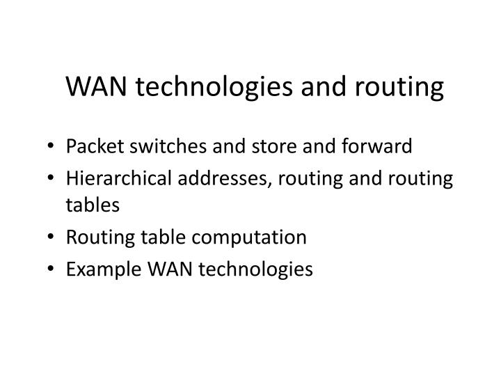
WAN technologies and routing. Packet switches and store and forward Hierarchical addresses, routing and routing tables Routing table computation Example WAN technologies. Categories of network technology. Local Area Network (LAN) Metropolitan Area Network (MAN) Wide Area network (WAN)

E N D
WAN technologies and routing • Packet switches and store and forward • Hierarchical addresses, routing and routing tables • Routing table computation • Example WAN technologies
Categories of network technology • Local Area Network (LAN) • Metropolitan Area Network (MAN) • Wide Area network (WAN) • Key distinguishing feature is scale: • geographic distance AND • number of connected computers
Packet Switches • In order to grow, WANs use many switches • Basic component is the packet switch that can connect to local computers and to other packet switches
WAN topology • Chosen to accommodate expected traffic and to provide redundancy
Store and forward • Each switch receives packets, queues them in its memory and then sends them out when possible (i.e., when the destination is available) • Many computers can send packets simultaneously
Physical addressing in a WAN • A WAN defines a frame format and assigns physical addresses to its computers • Hierarchical addressing, e.g., • first part identifies packet switch • second part identifies computer on this switch [2,2] [1,2] A C address [1,5] B [2,6] D switch 2 switch 1
Next hop forwarding • A packet switch determines the destination for each packet from the destination address • local computer or • another packet switch • Only has information about how to reach the next switch - next hop • This is held in a routing table
Example routing table [3,2] [1,2] Routing table for S2 Destination Next Hop [1,2] interface 1 [1,5] interface 1 [3,2] interface 4 [3,5] interface 4 [2,1] computer E [2,6] computer F C A S3 S1 B D [1,5] [3,5] S2 F E [2,6] [2,1]
Source independence • The next hop depends upon the destination address but not on the source address
Hierarchical addresses and routing • Routing is the process of forwarding a packet to its next hop • Hierarchical addresses simplify routing • smaller routing tables • more efficient look up
Routing in a WAN • Large WANs use interior switches and exterior switches • Their routing tables must guarantee that • Universal routing - there must be a next hop for every possible destination • Optimal routes - the next hop must point to the “shortest path” to the destination
Default routes • A routing table may be simplified by including (at most) one default route • Switch 1 • Destn next hop • - • * interface 3 • Switch 2 • Destn next hop • - • interface 4 • * interface 3 • Switch 3 • Destn next hop • 3 - • interface 2 • interface 3 • 4 interface 4
Routing table computation • Manual computation is not feasible for large networks • Static routing - program computes and installs routes when a switch boots; these routes do not change. • Dynamic routing - program builds an initial table when the switch boots; this alters as conditions change.
WANs and graphs • A Wan can be modelled as a graph • Nodes are switches: 1, 2, 3, 4 • Edges are connections between switches: (1,3) (2,3) (2,4) (3,4) • Weights are ‘distance’ along a connection
Computing the shortest path • Dijkstra’s algorithm - find the distance from a source node to each other node in a graph • Run this for each switch and create next-hop routing table as part of the process • “Distance” represented by weights on edges
Dijkstra’s algorithm • S = set of nodes, labelled with current distance from source, but for which minimum distance is not yet known • Initialise S to everything but the source • Iterate: • select the node, u, from S that has smallest current distance from source • examine each neighbour of u and if distance to the neighbour from source is less via u than is currently recorded in S then update
Implementation • Data structure to store information about the graph (nodes and edges) • Integer labels for the nodes [1..n] • Three data structures: • current distance to each node - array - D[1..n] • next hop destination for each node array - R[1..n] • set S of remaining nodes - linked list - S • weight(i, j) function (infinity if no edge)
Given: a graph with nonnegative weight assigned to each edge and a designated source node Compute: the shortest distance from the source node to each other node and a next-hop routing table Method: Initialise the set S to contain all nodes except the source Initialise D so that D[u] = weight(source, u) Initialise R so that R[v] = v if there is an edge from the source to v and zero otherwise
while ( set S is not empty ) { choose a node u from S such that D[u] is minimum if ( D[u] is infinity ) { error: no path exists to nodes in S; quit } delete u from set S for each node v such that (u, v) is an edge { if v still in S { c = D[u] + weight (u,v); if c < D[v] { R[v] = R[u] D[v] = c; } } } }
Example S = { 1, 2, 3, 4, 5, 6, 7 } Distance D 1 2 3 4 5 6 7 Next hop route R 1 2 3 4 5 6 7
Example S = source = 6 S = { 1, 2, 3, 4, 5, 6, 7 } Distance D 1 2 3 4 5 6 7 Next hop route R 1 2 3 4 5 6 7 ∞ 8 2 ∞ ∞ - 5 X 5 X 13 0 2 3 0 0 - 7 0 3 3 3 0 - 7
Distributed route computation • Dijkstra’s algorithm requires each switch to hold a complete description of the network • In distributed route computation computation, each switch periodically computes a new local table and sends it to its neighbours • After a while, the switches learn shortest routes or adapt to changes in the network
Given: a local routing table, a weight for each link that connects to another switch and an incoming routing message Compute: an updated routing table Method: maintain a distance field in each routing table entry initialise routing table with a single entry that has the destination equal to the local packet switch, the next hop unused and the distance set to sero
Repeat forever { wait for the next routing message to arrive over the network; let the sender be switch N for each entry in the message { let V be the destination in the entry and D the distance compute C as D plus the weight of the link over which the message arrived examine and update the local routing table { if ( no route exists to V ) { add an entry to the local table for V with next hop N and distance C } else if ( a route exists with next hop N ) { replace existing distance with C } else if (route exists with distance > C ) change next hop to N and distance to C } } }
Link state routing • Each switch periodically broadcasts state of specific links to other switches • Switches collect these messages and then apply Dijkstra’s algorithm to their version of the state of the network