Download
1 / 47
470 likes | 566 Views
Modeling the multivariate dynamical properties of spatially distributed data sets: the electrojet currents. J. A. Valdivia. Collaborators A. Klimas D. Vassiliadis S. Sharma K. Papadopoulos. Outline. Magnetospheric activity As an input-output system Time delay embeddings

E N D
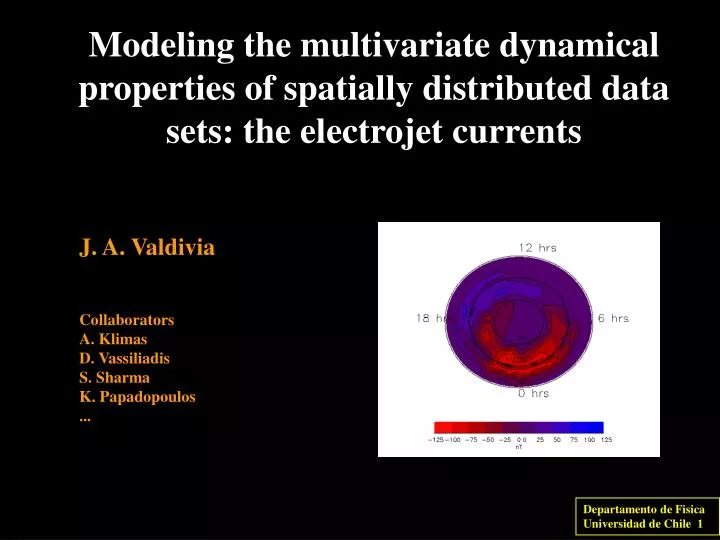
Modeling the multivariate dynamical properties of spatially distributed data sets: the electrojet currents J. A. Valdivia Collaborators A. Klimas D. Vassiliadis S. Sharma K. Papadopoulos ...
Outline • Magnetospheric activity • As an input-output system • Time delay embeddings • Dimensionality? • Singular value decomposition? • Modeling • Driven system • Modeling • Phase transitions? • Syncronization? • Other analyses • Modeling and prediction • Time delay embedding • Linear vs Nonlinear models • Nearest neighbors • Fuzzy Logic • Neural nets • Nonlinear analogues • Relation to physics • Systems with spatial structure • Ring current • High latitude magnetic perturbations • Applications • Space weather • Where are we going?
Motivation System Input Output Wiltberger et al Magnetosphere as an Input-output system The idea is to learn the properties of the system: relevant time scales, coupling coefficients. When the output represent spatial information (such as multiple magnetometer information) we can also learn the spatial modes of the system, transport, etc.
Motivation Input-output : Nonlinear transfer function More general methods to analyze Chaotic time series Catastrophe Time delay embeddings Spatiotemporal chaos Self organized criticality etc. Bargatze et al
PHASE SPACE TRAJECTORY O(t) O(t-t) Time delay embeddings Assume a phase space of dimension D=m+1 Theorem by Takens Hopefully defines an attractor for the dynamics system is spatio-temporal -> infinite modes system is driven
Dimensionality Now we hope to have an attractor: Invariant measure Dimension spectrum Suggest m ~ 3 but difficult to do because not clear what e to use The system is driven and very noisy, must be cleaned -> Singular value decomposition Vassiliadis et al
Singular value decomposition The system is driven and very noisy, must be cleaned Singular value decomposition Diagonalize cross-correlation matrix to find time uncorrelated eigenvectors The projection to this space is hopefully cleaner and capable of giving a D
Singular value decomposition The trajectories are cleaner, specially the 2nd and 3er components. The spectrum of singular values gives an indication of the importance of each eigendirection Suggest m ~ 3 Sharma et al Sharma et al
Going to Physics Attempts to derive low dimensional physics models Klimas et al., 1992 Horton and Doxas et al., 1992
Modeling If phase space concept makes sense (either X or Y=UX) Reconstruct evolution function Study dynamical properties Linear Model Ai= cons Non Linear Model Ai = f[X] Physics: Coefficients Ai can be transformed to standard parameters like time scales ti by transforming the above equation to a nonlinear ODE using Z-transforms Lyapunov Exponent: O(t) and O(t)+dO(t)
Driven System Include Input Issue of propagation -> Ballistic -> 1-D MHD -> use conserved propagation Is planar assumption truly realistic?
Phase transitions SVD + rotation 3 principal components Gives something that resembles a catastrophe -> controlled by solar wind input See a scaling that looks like a phase transition Sitnov et al
Modeling Linear ModelAi= const Bi= const Nonlinear ModelAi = f[X] Bi = g[X] PHYSICS:Coefficients Ai and Bi can be transformed to standard parameters like time scales ai and coupling coefficients bi by transforming the above equation to a nonlinear ODE using Z-transforms
I(t-tDt) O(t-tDt) Modeling Linear Model Ai= const Bi= const Local COM Local Linear/Nonlinear (+ SVD + other + neighborhood )
Modeling Fuzzy sets Neural Nets Closure relations
Synchronization Lyapunov Exponent: O(t) and O(t)+dO(t) If solar wind is a high dimensional system N of positive exponents N > mi Synchronization Driver Dynamical System Synchronize to a low dimensionality system if the reduced Lyapunov exponents are negative (possibly a chaotic system)
Synchronization Spectrum for Bargaze 31 Average spectrum Eventually synchronizes -> SOC? Need to look at local Lyapunov exponents
Other analysis Event distributions Self-organization?
PROBLEMS -> SO? III (5) Low dimensional Magnetospheric Dynamics (6) Energy output from Polar UVI images (Uritsky et al) (Liu et al, GRL 2000) (Liu et al, GRL 2000)
Continuous models? TO START: FROZEN IN and Beyond MHD B field is frozen with the plasma when Reconnection -> how the Frozen in condition is broken
Hysteresis Q(J) Dmax Dmin bk k Bx(z) z 0 Approximation 1-D Z
Approximation 1-D Reconnection (BBF) Chaos -> driver is constant in t Renormaliztion group & spatio-temporal chaos
I(t-tDt) O(t-tDt) Modeling Linear Model Ai= const Bi= const Local COM Local Linear/Nonlinear (+ SVD + other + neighborhood ) Closure relations
AL prediction using local linear Vassiliadis et al., JGR, 100, 3495-3512, 1995
Closure relations The process of obtaining the coefficients Ai and Bi PHYSICS:Coefficients Ai and Bi can be transformed to standard parameters like time scales ai and coupling coefficients bi by transforming the above equation to a nonlinear ODE using Z-transforms
Closure relations Can be written in analytical form in the limit For m = 2 and l = 1 we get Closure relation -> 6 constant coefficients (a0,0, a0,1, a1,0, a1,1, b0,0, b0,1, ) -> to integrate the equation forward in time.
Dst prediction using closure relations Training interval: for Dst a<<1 Out-of-sample prediction
Sign of loading-unloading The delayed driver (red curve on the VBs panel) shows that these closure relations have in them the physics of the loading-unloading processes.
AL prediction using closure relations Training interval: for AL a>1 Out-of-sample prediction
PHASE SPACE TRAJECTORY I(t-tDt) O(t-tDt) Spatial Structure Time delay embeddings: assume a phase space of dimension
I(t-tDt) O(t-tDt) Modeling Linear Model Ai= const Bi= const Local COM Local Linear/Nonlinear (+ SVD + other + neighborhood )
MLMP Extension to spatial data The idea is to model the Mid Latitude Magnetic Perturbations as measured by a set of magnetometers Dynamic ->Dt ~ 1min Small time steps Propagation very important
Compare Nonlinear models Predictions: Global vs spatial
12 6 12 0 1-D Extension to spatial data • The idea is to model the High Latitude Magnetic Perturbations as measured by a chain of magnetometers • Model the magnetic fluctuations as measured by the Magnetometer Array and its dependence in local time (MLT), i.e., “as it moves in local time”. • Dynamic ->Dt ~ 1min Small time steps • Propagation very important • Magnetometer Arrays: • IMAGE • CANOPUS • MM210
Canopus 1D example Model the magnetic fluctuations as measured by Canopus and its dependence in local time (MLT). Spatial dependence measured by the Canopus chain in latitude at the 4 times marked in above panel.
12 6 12 0 2-D Extension to spatial data • The idea is to model the 2D High Latitude Magnetic Perturbations as measured by an ensemble of virtual chains of magnetometers and the related current system • Model the magnetic fluctuations as measured by the Magnetometer Array and its dependence in local time (MLT). • Divide data into local time (MLT) bins. A different 1-D model is constructed in each bin, in practice generating a 2-D model by putting together an ensemble of magnetometer arrays • Magnetometer Arrays: • IMAGE • CANOPUS • MM210
2D Example: IMAGE 12 Ensemble of Virtual Magnetometer Arrays 6 12 12 0 Start with a “good guess” of the initial condition (average of all measurements with similar local times)
The Hx component The current structure
Evolution of 2D Model Whether this is a substorm or not will have to be determined by other means. But the model clearly shows an electrojet intensification that seems to have some of the features of a substorm. We must also compare the evolution of the pattern with magnetometers at other locations far from the IMAGE chain to check for the reliability of the model.
Evolution of 2D Model Whether this is a substorm or not will have to be determined by other means. But the model clearly shows an electrojet intensification that seems to have some of the features of a substorm. We must also compare the evolution of the pattern with magnetometers at other locations far from the IMAGE chain to check for the reliability of the model.
Evolution of 2D Model Dynamic ->Dt ~ 1min Small time steps Propagation very important Get latitudinal and longitudinal coverage -> mode dynamics Orthogonal expansion Spatial SVD expansion Constrained regression to satisfy Connect with an electrodynamica model Potential patterns Ionospheric currents Field aligned currents Space weather
Solar wind data from the ACE satellite Propagate to the subsolar point Simultaneous Data base (1995) Wind datellite data Image mag chain Nonlinear Dynamical Model Training data Nonlinear Model Construction of web page