Download
1 / 31
610 likes | 1.45k Views
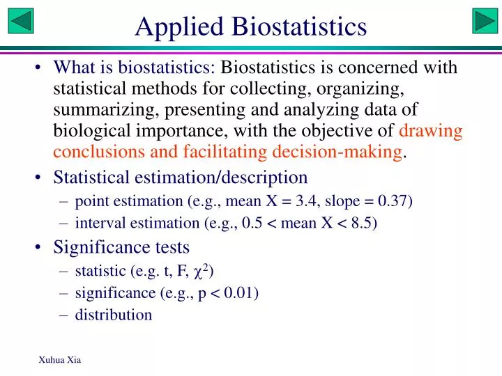
Applied Biostatistics. What is biostatistics: Biostatistics is concerned with statistical methods for collecting, organizing, summarizing, presenting and analyzing data of biological importance, with the objective of drawing conclusions and facilitating decision-making .

E N D
Applied Biostatistics • What is biostatistics: Biostatistics is concerned with statistical methods for collecting, organizing, summarizing, presenting and analyzing data of biological importance, with the objective of drawing conclusions and facilitating decision-making. • Statistical estimation/description • point estimation (e.g., mean X = 3.4, slope = 0.37) • interval estimation (e.g., 0.5 < mean X < 8.5) • Significance tests • statistic (e.g. t, F, 2) • significance (e.g., p < 0.01) • distribution
Decision making and risks Decision Accepted Rejected H0: Product is good True Correct Type I Error False Type II Error Correct 1. Type I error is also called Producer’s risk (rejecting a good product), and is typically represented by the Greek letter . 2. Type II error is often referred to as consumer’s risk (accepting an inferior product), and is typically represented by . One can avoid making Type II errors by making no decision (not accepting any hypothesis when the null hypothesis is not rejected). 3. The power of a test is 1- which depends on sample size and effect size.
Numbers and statistics • Issac Newton (1643 –1727): God created everything by number, weight and measure • Lord Kelvin (1824 –1907): When you can measure what you are speaking about, and express it in numbers, then you know something about it; but when you cannot measure it, when you cannot express it in numbers, your knowledge is of a meager and unsatisfactory kind. • Winston Churchill (1874 –1965): Surely the account you give of all these various disconnected statistical branches constitutes the case for a central body which should grip together all admiralty statistics and present them to me in a form increasingly simplified and graphic. I want to know at the end of each week everything we have got, all the people we are employing, the progress of all vessels, works of construction, the progress of all munitions affecting us, the state of our merchant tonnage, together with losses, and numbers of every branch of the Royal Navy and Marines. The whole should be presented in a small book such as was kept for me when Sir Walter Layton was my statistical officer at the Ministry of Munitions in 1917 and 1918. Every week I had this book, which showed the past and weekly progress, and also drew attention to what was lagging. In an hour or two I was able to cover the whole ground, as I know exactly what to look for and where. How do you propose this want of mine should be met? • Banjamin D’Israeli (1804 –1881): There are three types of lies: lies, damned lies, and statistics • Ernest Rutherford (1871–1937): If your experiment needs statistics, you should have done a better experiment.
Biostatistics and science Proportions of papers involving numerical and statistical work in decennial issues of The American Naturalist
Inference: Population and Sample Variable Variate ID Weight Length (in kg) (in m) 1 2.3 0.3 2 2.5 0.3 3 2.5 0.5 4 2.4 0.4 5 2.4 0.4 6 2.3 0.5 Mean 2.4 0.4 Population Sample Sample Individual Statistic Observation
Estimates and Sample Size Frequency distributions of sampling from a population with 10% HIV-1 carriers, with N = 10.
Essential definitions • Statistic: any one of many computed or estimated statistical quantities, such as the mean, the standard variation, the correlation coefficient between two variables, the t statistic for two-sample t-test. • Parameter: a numerical descriptive measure (attribute) of a population. • Population: a specified set of individuals (or individual observations) about which inferences are to be made. • Sample: a subset of individuals (or individual observations), generally used to make inference about the population from which the sample is taken from.
Elementary Probability Theory • Empirical probability of an event is taken as the relative frequency of occurrence of the event when the number of observations is very large. • A coin is tossed 10000 times, and we observed head 5136 times. The empirical probability of observing a head when a coin is tossed is then5136/10000 = 0.5136. • A die is tossed 10000 times and we observed number 2 up 1703 times. What is the empirical probability of getting a 2 when a die is tossed? • If the coin and the die are even, what is the expected probabilities for getting a head or a number 2?
Mutually Exclusive Events • Two or more events are mutually exclusive if the occurrence of one of them exclude the occurrence of others. • Example: • observing a head and observing a tail in a single coin tossing experiment • events represented by null hypothesis and the alternative hypothesis • being a faithful husband and having extramarital affairs. • Binomial distribution
Coin-Tossing Expt. If I ask someone to toss a coin 6 times and record the number of heads, and he comes back to tell me that the number of heads is exactly 3. If I ask him repeat the tossing experiment three more times, and he always comes back to say that the number of heads in each experiment is exactly 3. What would you think? Experiment Outcome (Number of Heads out of 6 Coin-tossing)1 32 33 34 3The probability of getting 3 heads out of 6 coin-tossing is 0.3125 for a fair coin following the binomial distribution (0.5 + 0.5)6, and the probability of getting this result 4 times in a roll is 0.0095. The person might not have done the experiment at all!
Thinking Critically Now suppose Mendel obtained the following results: Breeding Experiment Number of Round Seeds Number of Wrinkled Seeds1 21 72 24 83 18 6 Based on (0.75+0.25)n: P1 = 0.171883; P2 = 0.161041; P3 = 0.185257; P = 0.0051 Edwards, A. W. F. 1986. Are Mendel’s results really too close? Biol. Rev. 61:295-312.
Compound Event • A compound event, denoted by E1E2 or E1E2…EN, refers to the event when two or more events occurring together. • For independent events, Pr{E1E2} = Pr{E1}Pr{E2} • For dependent events, Pr{E1E2} = Pr{E1}Pr{E2|E1}
Probability of joined events • Criteria Prob. • Between 25 and 45 1/2 • Very bright 1/25 • Liberal 1/3 • Relatively nonreligious 2/3 • Self-supporting 1/2 • No kids 1/3 • Funny, sense of humor 1/3 • Warm, considerate 1/2 • Sexually assertive 1/2 • Attractive 1/2 • Doesn’t drink or smoke 1/2 • Is not presently attached 1/2 • Would fall in love quickly 1/5 • The probability of meeting such a person satisfying all criteria is 1/648,000, i.e., • if you meet one new candidate per day, it will take you, on the average, 1775 years to find your partner. • Fortunately, many criteria are correlated, e.g., a very bright adult is almost always self-supporting.
Conditional Probability • Let E1 be the probability of observing number 2 when a die is tossed, and E2 be the probability of observing even numbers. The conditional probability, denoted by Pr{E1|E2} is called the conditional probability of E1 when E2 has occurred. • What is the expected value for the conditional probability of P{E1|E2} with a fair die? • What is the expected value for the conditional probability of P{E2|E1}?
Independent Events • Two events (E1 and E2) are independent if the occurrence or non-occurrence of E1 does not affect the probability of occurrence of E2, so that Pr{E2|E1} = Pr{E2}. • When one person throw a coin in Hong Kong, and another person throw a die in US, the event of observing a head and the event of getting a number 2 can be assumed to be independent. • The event of grading students unfairly and the event of students making an appeal can be assumed to be dependent.
Descriptive Statistics • Normal distribution: • Central tendency • dispersion • skewness • kurtosis. • There are two SAS procedures that output descriptive statistics: • univariate and means. • Sample SAS program and output • Confidence Limits.
Normal Distribution -6 -4 -2 0 2 4 6 Confidence Limits: Mean ± t,N SE
Moments and distribution • The moment (mr) • The central moment (r) • The first moment is the arithmetic mean • The second central moment • is the population variance when N is equal to population size (typically assumed to be infinitely large) • is the sample variance when N = n-1 where n is sample size • Standardized moment (r) = the moment of the standardized x. • 1 = 0 • 2 = 1 • 3 is population skewness; the sample skewness is
Skewness Right-Skewed (+) Left-Skewed (-) -6 -4 -2 0 2 4 6
Kurtosis Leptokurtic(Kurtosis < 0) Normally distributed Platykurtic (Kurtosis > 0) -6 -4 -2 0 2 4 6
Various Kinds of Means • Arithmetic mean • Geometric mean • Harmonic mean • Quadratic mean (or root mean square)
Geometric Mean • The geometric mean (Gx) is expressed as: • where is called the product operator (and you know that is called the summation operator.
When to Use Geometric Mean • The geometric mean is frequently used with rates of change over time, e.g., the rate of increase in population size, the rate of increase in wealth. • Suppose we have a population of 1000 mice in the 1st year (x1 = 1000), 2000 mice the 2nd year (x2 = 2000), 8000 mice the 3rd year (x3 = 8000), and 8000 mice the 4th year (x4 = 8000). This scenario is summarized in the following table: What is the mean rate of increase? (2+4+1) / 3 ?
Wrong Use of Arithmetic Mean • The arithmetic mean is (2+4+1) / 3 = 7/3, which might lead us to conclude that the population is increasing with an average rate of 7/3. • This is a wrong conclusion because1000 * 7/3 * 7/3 * 7/3 8000 • The arithmetic mean is not good for ratio variables.
Using Geometric Mean • The geometric mean is: • This is the correct average rate of increase. On average, the population size has doubled every year over the last three years, so that x4 = 1000 222 = 8000 mice. • Alternative: 1000*r3 = 8000
The Ratio Variable • Example: • Year 1: • Year 2: • The arithmetic mean ratio is r1 = 2.5 • What is the mean ratio of bread price to milk price? • Ratio1 = 1/3; Ratio2 = 1/2 • Mean ratio is r2 = (1/3 + 1/2) / 2 = 5/12 = 0.4167. • But r1 1/r2. What’s wrong? • Conclusion: Arithmetic mean is no good for ratios
Using Geometric Mean • Geometric mean of the milk/bread ratios: • Geometric mean of the bread/milk ratios:
Chest Number of Men(inches)33 334 1835 81 36 185 37 420 38 74939 1073 40 1079 41 934 42 658 43 370 44 92 45 50 46 21 47 4 48 1 Marks Number of (mid-point) candidates 400 24 750 74 1250 38 1750 21 2250 11 2750 8 3250 11 3750 5 4250 2 4750 1 5250 3 5750 1 6250 0 6750 0 7250 0 7750 1 Empirical frequency distributions
SAS Program and Output Univariate Procedure Variable=CHEST N 5738 Sum Wgts 5738 Mean 39.83182 Sum 228555 Std Dev 2.049616 Variance 4.200925 Skewness 0.03333Kurtosis 0.06109 USS 9127863 CSS 24100.71 CV 5.145674 Std Mean 0.027058 T:Mean=0 1472.102 Pr>|T| 0.0001 Num ^= 0 5738 Num > 0 5738 M(Sign) 2869 Pr>=|M| 0.0001 Sgn Rank 8232596 Pr>=|S| 0.0001 D:Normal 0.098317 Pr>D <.01 USS = Sum(xi2) CSS = Sum(xi – MeanX)2 data chest; input chest number; cards; 33 3 34 18 35 81 36 185 37 420 38 749 39 1073 40 1079 41 934 42 658 43 370 44 92 45 50 46 21 47 4 48 1 ; proc univariate normal plot; freq number; var chest; run;
SAS Program and Output data Grade; input marks number; cards; 400 24 750 74 1250 38 1750 21 2250 11 2750 8 3250 11 3750 5 4250 2 4750 1 5250 3 5750 1 6250 0 6750 0 7250 0 7750 1 ; proc univariate normal plot; freq number; var marks; run; Univariate Procedure Variable= marks N 200 Sum Wgts 200 Mean 1465.5 Sum 293100 Std Dev 1179.392 Variance 1390965 Skewness 2.031081 Kurtosis 5.180086 USS 7.0634E8 CSS 2.768E8 CV 80.47708 Std Mean 83.39558 T:Mean=0 17.57287 Pr>|T| 0.0001 Num ^= 0 200 Num > 0 200 M(Sign) 100 Pr>=|M| 0.0001 Sgn Rank 10050 Pr>=|S| 0.0001 W:Normal 0.767621 Pr<W 0.0001
SAS Graph DATA; DO X=-5 TO 5 BY 0.25; DO Y=-5 TO 5 BY 0.25; DO Z=SIN(SQRT(X*X+Y*Y)); OUTPUT; END; END; END; PROC G3D; PLOT Y*X=Z/CAXIS=BLACK CTEXT=BLACK; TITLE 'Hat plot'; FOOTNOTE 'Fig. 1, Xia'; RUN;