Download

1 / 97
980 likes | 1.14k Views
CS461: Artificial Intelligence. Lecture 6: Constraint Satisfaction Problems. Outline. Constraint Satisfaction Problems (CSP) Backtracking search for CSPs Local search for CSPs. Constraint satisfaction problems (CSPs). Standard search problem

E N D
CS461: Artificial Intelligence Computer Science Department Lecture 6: Constraint Satisfaction Problems
Outline • Constraint Satisfaction Problems (CSP) • Backtracking search for CSPs • Local search for CSPs Computer Science Department
Constraint satisfaction problems (CSPs) • Standard search problem • state is a "black box“ – any data structure that supports successor function, heuristic function, and goal test • CSP: • state is defined by variablesXi with values from domainDi • goal test is a set of constraints specifying allowable combinations of values for subsets of variables • Simple example of a formal representation language • Allows useful general-purpose algorithms with more power than standard search algorithms Computer Science Department
Example: Map-Coloring • VariablesWA, NT, Q, NSW, V, SA, T • DomainsDi = {red,green,blue} • Constraints: adjacent regions must have different colors • e.g., WA ≠ NT, or (WA,NT) in {(red,green),(red,blue),(green,red), (green,blue),(blue,red),(blue,green)} Computer Science Department
Example: Map-Coloring • Solutions are complete and consistent assignments, e.g., WA = red, NT = green,Q = red,NSW = green,V = red,SA = blue,T = green Computer Science Department
Constraint graph • Binary CSP: each constraint relates two variables • Constraint graph: nodes are variables, arcs are constraints Computer Science Department
Varieties of CSPs • Discrete variables • finite domains: • n variables, domain size d O(dn) complete assignments • e.g., Boolean CSPs, incl.~Boolean satisfiability (NP-complete) • infinite domains: • integers, strings, etc. • e.g., job scheduling, variables are start/end days for each job • need a constraint language, e.g., StartJob1 + 5 ≤ StartJob3 • Continuous variables • e.g., start/end times for Hubble Space Telescope observations • linear constraints solvable in polynomial time by linear programming Computer Science Department
Varieties of constraints • Unary constraints involve a single variable, • e.g., SA ≠ green • Binary constraints involve pairs of variables, • e.g., SA ≠ WA • Higher-order constraints involve 3 or more variables, • e.g., cryptarithmetic column constraints Computer Science Department
Real-world CSPs • Assignment problems • e.g., who teaches what class • Timetabling problems • e.g., which class is offered when and where? • Transportation scheduling • Factory scheduling • Notice that many real-world problems involve real-valued variables Computer Science Department
Standard search formulation (incremental) Let's start with the straightforward approach, then fix it States are defined by the values assigned so far • Initial state: the empty assignment { } • Successor function: assign a value to an unassigned variable that does not conflict with current assignment fail if no legal assignments • Goal test: the current assignment is complete • This is the same for all CSPs • Every solution appears at depth n with n variables use depth-first search • Path is irrelevant, so can also use complete-state formulation • b = (n - l )d at depth l, hence n! · dn leaves Computer Science Department
NxD WA WA WA NT T [NxD]x[(N-1)xD] WA NT WA NT WA NT NT WA Standard search formulation N layers Equal! N! x DN There are N! x DN nodes in the tree but only DN distinct states?? Computer Science Department
Backtracking search • Variable assignments are commutative}, i.e., [ WA = red then NT = green ] same as [ NT = green then WA = red ] • Only need to consider assignments to a single variable at each node • Depth-first search for CSPs with single-variable assignments is called backtracking search • Backtracking search is the basic uninformed algorithm for CSPs • Can solve n-queens for n ≈ 25 Computer Science Department
D WA WA WA WA NT D2 WA NT WA NT DN Backtracking search Computer Science Department
function BACKTRACKING-SEARCH (csp) returns a solution, or failure return RECURSIVE-BACKTRACKING({}, csp) function RECURSIVE-BACKTRACKING(assignment, csp) returns a solution, or failure ifassignment is complete then returnassignment var SELECT-UNASSIGNED-VARIABLE(VARIABLES[csp], assignment, csp) for eachvalue in ORDER-DOMAIN-VALUES(var, assignment, csp) do ifvalue is consistent with assignment according to CONSTRAINTS[csp] then add {var=value} to assignment result RECURSIVE-BACKTRACKING(assignment, csp) ifresult != failurethen returnresult remove {var = value} from assignment return failure ☜ BACKTRACKING OCCURS HERE!! Backtracking search Computer Science Department
Backtracking example Computer Science Department
Backtracking example Computer Science Department
Backtracking example Computer Science Department
Backtracking example Computer Science Department
Improving backtracking efficiency • General-purpose methods can give huge gains in speed: • Which variable should be assigned next? • In what order should its values be tried? • Can we detect inevitable failure early? Computer Science Department
Most constrained variable • Most constrained variable: choose the variable with the fewest legal values • a.k.a. minimum remaining values (MRV) heuristic Computer Science Department
BackpropagationMRVminimum remaining values • choose the variable with the fewest legal values Computer Science Department
Backpropagation - MRV [R,B,G] [R,B,G] [R] [R,B,G] [R,B,G] Computer Science Department
Backpropagation - MRV [R,B,G] [R,B,G] [R] [R,B,G] [R,B,G] Computer Science Department
Backpropagation - MRV [R,B,G] [R,B,G] [R] [R,B,G] [R,B,G] Computer Science Department
Backpropagation - MRV [R,B,G] [R,B,G] [R] [R,B,G] [R,B,G] Computer Science Department
Backpropagation - MRV [R,B,G] [R,B,G] [R] [R,B,G] [R,B,G] Computer Science Department
Backpropagation - MRV [R,B,G] [R,B,G] [R] [R,B,G] [R,B,G] Solution !!! Computer Science Department
Most constraining variable • Tie-breaker among most constrained variables • Most constraining variable: • choose the variable with the most constraints on remaining variables (most edges in graph) Computer Science Department
Backpropagation - MCV [R,B,G] [R,B,G] 4 arcs 2 arcs 2 arcs [R] 3 arcs 3 arcs [R,B,G] [R,B,G] Computer Science Department
Backpropagation - MCV [R,B,G] [R,B,G] 4 arcs 2 arcs 2 arcs [R] 3 arcs 3 arcs [R,B,G] [R,B,G] Computer Science Department
Backpropagation - MCV [R,B,G] [R,B,G] 4 arcs 2 arcs 2 arcs [R] 3 arcs 3 arcs [R,B,G] [R,B,G] Computer Science Department
Backpropagation - MCV [R,B,G] [R,B,G] 4 arcs 2 arcs 2 arcs [R] 3 arcs 3 arcs [R,B,G] [R,B,G] Computer Science Department
Backpropagation - MCV [R,B,G] [R,B,G] 4 arcs 2 arcs 2 arcs [R] 3 arcs Dead End 3 arcs [R,B,G] [R,B,G] Computer Science Department
Backpropagation - MCV [R,B,G] [R,B,G] 4 arcs 2 arcs 2 arcs [R] 3 arcs 3 arcs [R,B,G] [R,B,G] Computer Science Department
Backpropagation - MCV [R,B,G] [R,B,G] 4 arcs 2 arcs 2 arcs [R] 3 arcs 3 arcs [R,B,G] [R,B,G] Computer Science Department
Backpropagation - MCV [R,B,G] [R,B,G] 4 arcs 2 arcs 2 arcs [R] 3 arcs 3 arcs [R,B,G] [R,B,G] Computer Science Department
Backpropagation - MCV [R,B,G] [R,B,G] 4 arcs 2 arcs 2 arcs [R] 3 arcs 3 arcs [R,B,G] [R,B,G] Computer Science Department
Backpropagation - MCV [R,B,G] [R,B,G] 4 arcs 2 arcs 2 arcs [R] 3 arcs 3 arcs [R,B,G] [R,B,G] Solution !!! Computer Science Department
Least constraining value • Given a variable, choose the least constraining value: • the one that rules out the fewest values in the remaining variables • Combining these heuristics makes 1000 queens feasible Computer Science Department
Back-propagation LCV [R,B,G] [R,B,G] 4 arcs 2 arcs 2 arcs [R] 3 arcs 3 arcs [R,B,G] [R,B,G] Computer Science Department
Back-propagation LCV [R,B,G] [R,B,G] 4 arcs 2 arcs 2 arcs [R] 3 arcs 3 arcs [R,B,G] [R,B,G] Computer Science Department
Back-propagation LCV [R,B,G] [R,B,G] 4 arcs 2 arcs 2 arcs [R] 3 arcs 3 arcs [R,B,G] [R,B,G] Computer Science Department
Back-propagation LCV [R,B,G] [R,B,G] 4 arcs 2 arcs 2 arcs [R] 3 arcs 3 arcs [R,B,G] [R,B,G] Computer Science Department
Back-propagation LCV [R,B,G] [R,B,G] 4 arcs 2 arcs 2 arcs [R] 3 arcs 3 arcs [R,B,G] [R,B,G] Computer Science Department
Back-propagation LCV [R,B,G] [R,B,G] 4 arcs 2 arcs 2 arcs [R] 3 arcs 3 arcs [R,B,G] [R,B,G] Dead End Computer Science Department
Back-propagation LCV [R,B,G] [R,B,G] 4 arcs 2 arcs 2 arcs [R] 3 arcs 3 arcs [R,B,G] [R,B,G] Computer Science Department