Download
1 / 15
150 likes | 288 Views
Production Information and Decision Systems Final Presentation. Utility Theory 在半導體產能決策模式之應用. 指導老師:周雍強教授 小組成員:吳全順、陳昭任. Goal :計算 Optimal Operation Point. Indifference Curve. Cycle Time (better >). Optimal Operation Point. Option Curve. Throughput (better >). 求解方法概觀.

E N D
Production Information and Decision Systems Final Presentation Utility Theory 在半導體產能決策模式之應用 指導老師:周雍強教授 小組成員:吳全順、陳昭任
Goal:計算 Optimal Operation Point Indifference Curve Cycle Time (better >) Optimal Operation Point Option Curve Throughput (better >)
求解方法概觀 求出Option Curve的近似函數 根據一組Throughput及 Cycle Time的Data,依迴歸得到一條連續函數oc(x) 求出總效用函數 透過定義Throghput效用函數、Cycle Time效用函數及權重W 以總效用函數為目標式,oc(x)為限制式,套用Lagrange乘數定理求得最佳解
將 Queuing Capacity Model 所得到的數據正規化,得到如下的 scatter diagram ,作為非線性迴歸的計算依據 Cycle Time (better >) Throughput (better >)
非線性迴歸的函數比較概觀 利用最小平方法,分別對以下四類型的函數進行迴歸 • 二次多項式 • 三次多項式 • 四次多項式 • 指數函數
非線性迴歸:二次多項式 結果: 缺點: 1. MSE = 0.053399 2. 明顯看出與實際資料有差異 3.不符合 Option Curve 遞減的特性 Cycle Time (better >) Throughput (better >)
非線性迴歸:三次多項式 結果: 缺點: 1. MSE = 0.011198 2.左上角曲線落有明顯上升趨勢 ,但實際資料卻無此情形 Cycle Time (better >) Throughput (better >)
非線性迴歸:四次多項式 結果: 缺點: 1. MSE = 0.002379 2. 參數高達五個,敏感度太高 Cycle Time (better >) Throughput (better >)
非線性迴歸:指數函數 結果: 優點: 1.MSE = 0.0099569 2.要決定參數較少,敏感度較低 Cycle Time (better >) Throughput (better >)
定義總效用函數 Throughput 效用函數 UTH = Cycle Time 效用函數 UCT = 相對權重係數: 總效用函數 U =
總效用函數之曲面及等高線 Indifference Curves Option Curve
Lagrange 乘數定理之應用 目標函數:=總效用函數 U(x,y) 限制等式:= OCE(x,y) = 0 = OC(x) - y Lagrange函數 由下列的聯立方程式解出 x, y : • 要注意的是: • 解(x,y)可能有一組以上 • 當有 m 個變數及 n 個限 制式,此方法仍適用
Optimal Operation Point 計算結果 正規化依據點: Throughput (ST) = 8760 wafers (SA) =13080 wafers Cycle Time (ST) = 2009.40 hours (SA) = 591.06 hours Optimal operation point (x,y)=(0.68,0.69) 實際最佳操作點: Throughput = ST + x * ( ST – SA ) = 11770.61 wafers Cycle Time = ST – y * ( ST – SA ) = 1040.80 hours
另一種求解方法:連鎖律與一階導數之應用 Let y=OC(x) be option curve Let u(x)=U(x,y)=U(x,OC(x))=UTH(x)+UCT(OC(x)) By Chain Rule Let Solve x first, then compute y and U by OC(x) and U(x,y) respectively
結論 • 我們找到兩種方法: • Lagrange 乘數 • 連鎖律及一階導數 都可以求得 Optimal Operation Point