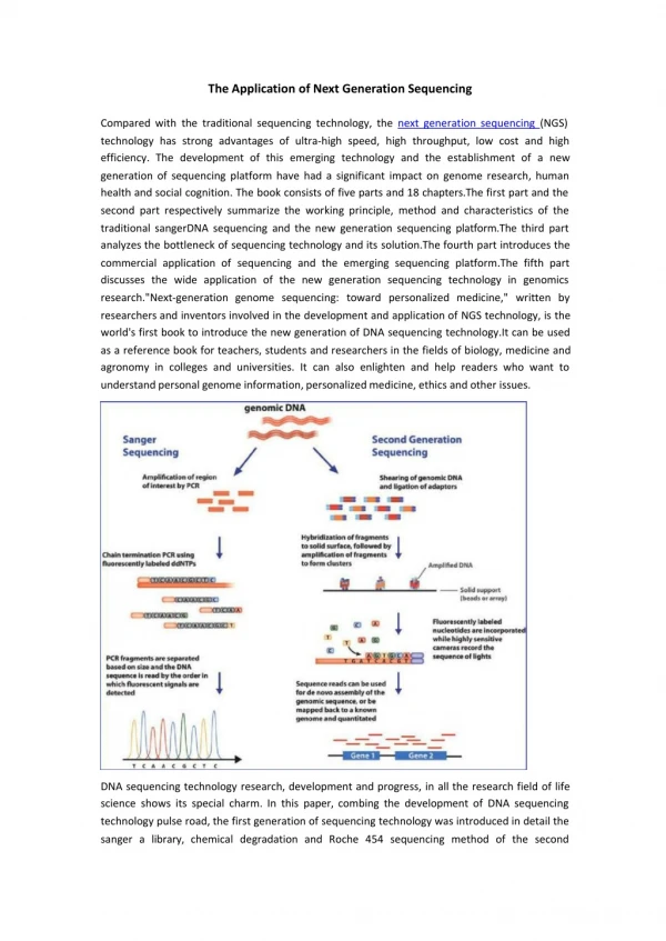
Download
1 / 32
320 likes | 433 Views
Amplicon -Based Quasipecies Assembly Using Next Generation Sequencing. Nick Mancuso Bassam Tork Computer Science Department Georgia State University. Outline of HCV Quasispecies. HCV quasispecies Problem formulation Amplicon based model Error model Frequency model Solution method

E N D
Amplicon-Based Quasipecies Assembly Using Next Generation Sequencing Nick Mancuso BassamTork Computer Science Department Georgia State University
Outline of HCV Quasispecies • HCV quasispecies • Problem formulation • Amplicon based model • Error model • Frequency model • Solution method • Goal
Outline of HCV Quasispecies – cont. • Optimization formulation (most parsimonious solution) • Quasispecies assembly in the error-free ideal-frequency model. • A case of two distinct reads for both amplicons • Read graph • Algorithm • Experiments
HCV Quasispecies • Many viruses (e.g., HCV) encode their genome in RNA rather than DNA. • RNA viruses are unable to detect and repair mistakes during replication due to the lack of DNA polymerase. • Mutations are passed down to descendants, producing a family of related variants of the ancestral genome referred as a quasispecies.
Problem Formulation • Given • A collection of 454 reads taken from a quasispecies population of unknown size and distribution, reference sequence • Assemble • Quasispecies sequences and estimate their frequencies.
Amplicon-Based Model • The amplicon-based quasipecies assembly covers the full virus genome with the collection of K sets over predefined positions within the genome, called amplicons. • Each amplicon A1, …, AK are sequenced to the same depth D. All reads over the amplicons have the same length.
Error Model We distinguish two error models: • Error-freemodel assumes that all reads are typing error-free or, equivalently, have been previously cleaned from typing errors and • Error-pronemodel allowssome typing errors and additionally these errors should be detected and fixed.
Frequency Model We distinguish two frequency models: • Ideal-frequency model assumes that in each amplicon distribution of reads is identical and equal to the true distribution of quasispecies • Skewed-frequency model assumes that in each amplicon the quasispecies are represented slightly different from the true distribution. It much closer reflects realistic scenarios.
Goal • The main goal is to reconstruct the genome-length quasispecies from amplicon data consisting of K x D reads. • The secondary goal is to optimize the amplicon based assembly parameters K, D and amplicon positions in order to maximize the quality (sensitivity and specificity) of assembly.
Goal • We also want to compare the amplicon-based and the shotgun sequencing approaches to quasispecies assembly. • Note that shotgun sequencing is more prone to typing errors but less prone to frequency skewing than amplicon based sequencing
Optimization formulation (most parsimonious solution) • We want to find minimum number of quasispecies explaining the observed reads • We also want to compare the amplicon-based and the shotgun sequencing approaches to quasispecies assembly. • Note that shotgun sequencing is more prone to typing errors but less prone to frequency skewing than amplicon based sequencing
Quasispecies Assembly in the Error-Free Ideal-Frequency Model • Given K amplicons A1, …, AK sequenced to the depth D, we need to assemble the most likely full-length quasispecies and find their frequency distribution. • K-staged read graph G=(V=V1 ∪ …∪ VK, E), where • ∀ v ∈ Vi corresponds to a distinct read in the i-th amplicon Ai and has a count c(v). • ∀ e=(u,v) ∈ E connects two reads from consecutive amplicons Ai and Ai+1 which agree in the overlap region.
Quasispecies Assembly in the Error-Free Ideal-Frequency Model – cont. • The solution can be viewed as the set Q={qj} of u-v-paths, uϵV1 , vϵVK, each with the frequency fj such that for each vertex vϵV, (1) • Rather than to solve the K-staged assembly problem, let’s focus on the 2-staged case whose solution can be further used to stitch together all K stages. • So we assume that there are only two stages V1 and V2 and therefore the read graph is bipartite.
Quasispecies Assembly in the Error-Free Ideal-Frequency Model – cont. Need to answer these 3 interconnected questions • Does a feasible solution exist? • How many quasispecies are there? • What is the most likely solution?
Does a feasible solution exist? • Let fe be the frequency of the quasispecies e corresponding to the edge e=(u,v). Then for each vertex we write the following constraint obtaining the following system of linear equations: • The above system of equations is consistent iff the 2-stage Assembly Problem is feasible.
How manyquasispecies are there? • The system may not have full rank and, therefore, the number of distinct quasispecies (or edges with non-zero frequency) in a feasible solution can be less than the total number of edges.
What is the most likely solution? • A simple maximum likelihood approach will assume that any edge (per single read) is equally probable. • That will not give us a correct assembly since it will try to assign non-zero frequency to all possible quasispecies, i.e., edges.
What is the most likely solution? • From the parsimonious principle we suggest to assume that only solutions with the minimum number of quasispecies should be considered. • A plausible approach would be first find all minimal solutions to the proposed system and then among them choose the one with the maximum likelihood.
The Case of Two Distinct Reads for Both Amplicons • Assume that |V1|=|V2|=2, A and B are distinct reads in the first amplicon and C and D are in the second. • Let all 4 possible combinations are consistent, i.e. common overlap is the same.
The Case of Two Distinct Reads for Both Amplicons • W.L.O.G. assume, that d ≦ b ≦ a ≦ c. If a = c, then b = d and we can have the minimum possible number of 2 non-zero edge frequencies. If a ≠ c, then the 4 constraints have rank 3 and there should be 3 edges with non-zero frequency.
The Case of Two Distinct Reads for Both Amplicons • There are two possibilities for 3 non-zero frequency edges: • AC = a, AD = 0, BC = c - a, and BD = d • AC = a - d, AD = d, BC = b, and BD = 0 • The first case is more probable if a > b and are equally probable if a = b.
Read Graph • Graph should be directed (left-to-right) • A single source S is added and is connected with all reads in the first amplicon. • A single sink T is added with edges from all reads in the last amplicon linked to it. • Each vertex v (except source/sink) split into two V1 V2: -->V--> replace with --->V1->V2--> all incoming to V will go to V1, all outgoing from V go to V2. • Edge V1->V2 has capacity c= frequency of V • Each original edge e has capacity xe which will be assigned infinity
Algorithm • Construct the matrix M where each column represents a multinomial distribution of distinct reads for each amplicon. • The multinomial distributions are all ordered decreasingly, as –for instance- in the following table (generated by 1,000 read samples)
Algorithm-cont. • In this example amplicon no. 7 has 10 distinct reads with frequencies {175, 173, 141, 116, 115, 95, 79, 44, 19}. • This may signify that (in an ideal case) there are exactly 10 variants in the quasispecies. • Note that in the table zero-frequencies are assumed where the number of distinct reads in one amplicon is below the maximum.
Algorithm-cont. • We choose now a guide distribution (say, the one corresponding to amplicon no. 7). • From this guide distribution we try to reconstruct a variant by starting from the most frequent read (7.a, n=175)
Algorithm-cont. • Checking if there is a consistent overlap among the other most frequent reads of each amplicon. • i.e. 6.a, 5.a, 4.a, 3.a, 2.a, 1.a (n=355, 185, 188, 312, 597, 773). If, among this first set of reads, there is one non-consistent overlap (say, with 2.a) we pass to the next read (which is 2.b).
Algorithm-cont. Suppose that we get all consistent overlaps for the read sets • (773) of amplicon no. 1 (first read, 1.a) • (132) of amplicon no. 2 (third read, 2.c) • (191) of amplicon no. 3 (second read, 3.b) • (188) of amplicon no. 4 (first read, 4.a) • (183) of amplicon no. 5 (second read, 5.b) • (355) of amplicon no. 6 (first read, 6.a) • (175) of amplicon no. 7 (first read, 7.a)
Algorithm-cont. • Every time that a virus is reconstructed, we subtract the number of reads of the guide distribution from the other reads that were selected (i.e. had consistent overlap). • Since the guide distribution is from amplicon no. 7, we subtract 175 from each one of the selected reads and get this table. • Again, a new guide distribution must be chosen and the whole procedure has to be repeated.
Thank you! Questions?