Download
1 / 8
80 likes | 87 Views
Learn about annuities, payment intervals, present value, accumulated value, and how to calculate payments for different annuity types.

E N D
Sections 3.1, 3.2, 3.3 A series of payments made at equal intervals of time is called an annuity. An annuity where payments are guaranteed to occur for a fixed period of time is called an annuity-certain. Unless otherwise indicated, this is the type of annuity we will assume, and the “certain” will be dropped from the name. An annuity where payments occur only under certain conditions is called an annuity-contingent. The interval between annuity payments is called an payment period, often just called a period.
An annuity under which payments of 1 are made at the end of each of period for n periods is called an annuity-immediate. Payments 1 1 1 1 Periods 0 1 2 … n– 1 n The present value of the annuity at time 0 is denoted , where the interest rate i is generally included only if not clear from the context. The accumulated value of the annuity at time n is denoted , where the interest rate i is generally included only if not clear from the context. a – n|i s – n|i = v + v2 + … + vn = = (1 + i)n–1 + (1 + i)n–2 + … + 1 = a – n| s – n| 1 – vn v—— = 1 – v 1 – vn —— i (1 + i)n– 1 ———— = (1 + i) – 1 (1 + i)n– 1 ———— i Values for and appear in Appendix I. a – n| s – n|
1 – vn = —— i 1 = i + vn a – n| a – n| The right hand side can be interpreted as the sum of the “present value of the interest payments” and the “present value of 1 (the original investment)” (1 + i)n– 1 = ———— i 1 = i + (1 + i)n s – n| s – n| One of the exercises asks you make a similar interpretation of this equation. Observe that = (1 + i)n s – n| a – n| 1 —— + i = i ———— + i = (1 + i)n– 1 i(1 + i)n ———— = (1 + i)n– 1 i —— = 1 – vn 1 —— Also, s – n| a – n| This identity will be important in a future chapter.
Find the present value of an annuity which pays $200 at the end of each quarter-year for 12 years if the rate of interest is 6% convertible quarterly. 200 = $6808.51 a –– 48 | 0.015 An investment of $5000 at 6% convertible semiannually. How much can be withdrawn each half-year to use up the fund exactly at the end of 20 years? Let R be the amount withdrawn (i.e., the payments) at each half-year. The present value at the time the investment begins is $5000, so the equation of value is 5000 = R R = $216.31 a –– 40 | 0.03
Compare the total amount of interest that would be paid on a $3000 loan over a 6-year period with an effective rate of interest of 7.5% per annum, under each of the following repayment plans: (a) (b) (c) The entire loan plus accumulated interest is paid in one lump sum at the end of 6 years. 3000(1.075)6 = $4629.90 Total Interest Paid = $1629.90 Interest is paid each year as accrued, and the principal is repaid at the end of 6 years. Each year, the interest on the loan is 3000(0.075) = $225 Total Interest Paid = $1350 The loan is repaid with level payments at the end of each year over the 6-year period. Let R be the level payments. 3000 = R R = $639.13 a –– 6 | 0.075 Total Interest Paid = 6(639.13) – 3000 = $834.78
An annuity under which payments of 1 are made at the beginning of each period for n periods is called an annuity-due. Payments 1 1 1 1 Periods 0 1 2 … n– 1 n The present value of the annuity at time 0 is denoted , where the interest rate i is generally included only if not clear from the context. The accumulated value of the annuity at time n is denoted , where the interest rate i is generally included only if not clear from the context. .. a – n|i .. s – n|i .. a – n| .. s – n| = 1 + v + v2 + … + vn–1 = = (1 + i)n + (1 + i)n–1 + … + (1 + i) = 1 – vn —— = 1 – v 1 – vn —— d (1 + i)n– 1 (1 + i) ———— = (1 + i) – 1 (1 + i)n– 1 ———— d
.. s – n| .. a – n| = Observe that (1 + i)n 1 —— + d = 1 —— This identity will be proven as an exercise. .. s – n| .. a – n| Also, .. a – n| In addition, observe that = (1 + i) a – n| .. s – n| = (1 + i) s – n| .. a – n| = 1 + a ––– n–1| .. s – n| = – 1 s ––– n+1| .. s – n| .. a – n| These last four formulas are useful, since values for and do not appear in most interest tables, including Appendix I.
An investor wishes to accumulate $3000 at the end of 15 years in a fund which earns 8% effective. To accomplish this, the investor plans to make deposits at the end of each year, with the final payment to be made one year prior to the end of the investment period. How large should each deposit be? Let R be the payments each year. The accumulated value of the investment at the end of the investment period is to be $3000, so the equation of value is .. s –– 14 | 0.08 3000 ———— = 3000 —————— = 3000 = R R = .. s –– 14 | 0.08 s –– 15 | 0.08 – 1 3000 ——— = 26.1521 $114.71