Classification and Prediction in Data Mining
710 likes | 731 Views
Learn about the concepts of classification and prediction in data mining, including decision tree induction, Bayesian classification, neural networks, and support vector machines. Explore topics like deep learning and classification accuracy.

Classification and Prediction in Data Mining
E N D
Presentation Transcript
CIS453/553, Spring 2018Data Mining Instructor: Dejing Dou Office hours: Mondays 4:00pm-5:00pm May 9 and May 11, 2018
Chapter 8,9: Classification and Prediction • What is classification? What is prediction? • Issues regarding classification and prediction • Classification by decision tree induction • Bayesian Classification • Classification by Neural Networks • Classification based on concepts from association rule mining • Support Vector Machine • Deep Learning • Prediction • Classification accuracy
Neural Networks • Analogy to Biological Systems (Indeed a great example of a good learning system) • Massive Parallelism allowing for computational efficiency • The first learning algorithm came in 1959 (Rosenblatt) who suggested that if a target output value is provided for a single neuron with fixed inputs, one can incrementally change weights to learn to produce these outputs using the perceptron learning rule
A Neuron • A cell in brain which can collect, process and disseminate electrical signals
A Simple Mathematical Model ai = g(jn=0 Wj,iaj)
Two activation functions • (a) Threshold function: outputs 1 when the input is positive and 0 otherwise • (b) Sigmoid function: 1/(1 + e-x), which is differentiable • The bias weight W0,i sets the actual threshold for the unit.
Perceptron vs. decision tree a0= -1 a1 W0 • A majority function (outputs 1 only if more than half of its n inputs are 1) can be a perceptron network with some Wj and W0, what they are? • A decision tree needs O(2n) nodes to represent this function . . . an Wj
Network Training • The ultimate objective of training • obtain a set of weights that makes almost all the tuples in the training data classified correctly • Steps • Initialize weights with random values • Feed the input tuples into the network one by one • For each unit • Compute the net input to the unit as a linear combination of all the inputs to the unit • Compute the output value using the activation function • Compute the error • Update the weights and the bias
Neural Network Learning • General idea: adjust the weights of the network to minimize some measure of the error on the training set. • So neural network learning can be formulated as an optimization search in weight space. • The “classical” measure of error is the sum of squared errors.
The squared error vs. weights The Squared Error: E = ½ Err2 = ½ (y - g(jn=0 Wjxj))2 We can use gradient descent to reduce the squared error by calculating the partial derivative of E respect to each weight: E/Wj = Err Err/Wj = Err (y – g(jn=0 Wjxj))/ Wj = - Err g’(in) xj where g’ is the derivative of the activation function. For sigmoid, g’ = g(1-g)
Weights updating If we want to reduce E, we can update the weights: Wj <= Wj + Err g’(in) xj is the learning rate. If the Err is positive, it means that output is too small. Then the weights are increased for the positive inputs and decreased for the negative inputs. The opposite happens when the error is negative.
Back Propagation Let Erri be ith component of the error vector y - hw(x) . Define i = Err g’(in), so the weight update rule for output layer is: Wj,i <= Wj,i + i aj The hidden node j is “responsible” for some faction of the error i in each of the output nodes to which it connects.
Back Propagation The i Values are divided according to the strength of connection between the hidden node and the output node and are propagated back to provide j values for the hidden layer: j = g’(in) Wj,i i Wk,j <= Wk,j + j ak By using math, we get: E/Wj,i = - aj i E/Wk,j = - ak j
Back Propagation It can be summarized as follows: • Compute the values for the output units, using the observed errors. • Starting with the output layer, repeat the following for each layer in the network, until the earliest hidden layer is reached • Propagate the values back to the previous layer • Update the weights between the two layers
Association-Based Classification • Several methods for association-based classification • ARCS: Quantitative association mining and clustering of association rules (Lent et al’97) • Mines association rules of form Aquan1^ Aquan2 => Acat • It beats C4.5 in (mainly) scalability and also accuracy • Associative classification: (Liu et al’98) • It mines high support and high confidence rules in the form of “cond_set => y”, where y is a class label • CAEP (Classification by aggregating emerging patterns) (Dong et al’99) • Emerging patterns (EPs): the itemsets whose support increases significantly from one class to another. E.g. {age =“ <=30”, student =“ no”} => buy_computer(Y/N): 0.2%/57.6% • Mine Eps based on minimum support and growth rate
SVM—Support Vector Machines • A new classification method for both linear and nonlinear data • It uses a nonlinear mapping to transform the original training data into a higher dimension • With the new dimension, it searches for the linear optimal separating hyperplane (i.e., “decision boundary”) • With an appropriate nonlinear mapping to a sufficiently high dimension, data from two classes can always be separated by a hyperplane • SVM finds this hyperplane using support vectors (“essential” training tuples) and margins (defined by the support vectors)
SVM—History and Applications • Vapnik and colleagues (1992)—groundwork from Vapnik & Chervonenkis’ statistical learning theory in 1960s • Features: training can be slow but accuracy is high owing to their ability to model complex nonlinear decision boundaries (margin maximization) • Used both for classification and prediction • Applications: • handwritten digit recognition, object recognition, speaker identification, benchmarking time-series prediction tests
Perceptron Revisited: Linear Separators • Binary classification can be viewed as the task of separating classes in feature space: wTx + b = 0 wTx + b > 0 wTx + b < 0 f(x) = sign(wTx + b)
Linear Separators • Which of the linear separators is optimal?
Small Margin Large Margin Support Vectors SVM—General Philosophy
SVM—When Data Is Linearly Separable r Let data D be (X1, y1), …, (X|D|, y|D|), where Xi is the set of training tuples associated with the class labels yi There are infinite lines (hyperplanes) separating the two classes but we want to find the best one (the one that minimizes classification error on unseen data) SVM searches for the hyperplane with the largest margin, i.e., maximum marginal hyperplane (MMH)
Classification Margin • Distance from example xi to the separator is • Examples closest to the hyperplane are support vectors. • Marginρ of the separator is the distance between support vectors. • Maximizing Margins implies that only support vectors matter; other training examples are ignorable. ρ r
SVM—Linearly Separable • A separating hyperplane can be written as W ● X + b = 0 where W={w1, w2, …, wn} is a weight vector and b a scalar (bias) • For 2-D it can be written as w0 + w1 x1 + w2 x2 = 0 • The hyperplane defining the sides of the margin: H1: w0 + w1 x1 + w2 x2 ≥ 1 for yi = +1, and H2: w0 + w1 x1 + w2 x2 ≤ – 1 for yi = –1 • Any training tuples that fall on hyperplanes H1 or H2 (i.e., the sides defining the margin) are support vectors • This becomes a constrained (convex) quadratic optimization problem: Quadratic objective function and linear constraints Quadratic Programming (QP) Lagrangian multipliers
Linear SVM Mathematically • Let training set {(xi, yi)}i=1..n, xiRd, yi{-1, 1}be separated by a hyperplane withmargin ρ. Then for each training example (xi, yi): • For every support vector xs the above inequality is an equality. After rescaling w and b by ρ/2in the equality, we obtain that distance between each xs and the hyperplane is • Then the margin can be expressed through (rescaled) w and b as: wTxi+ b ≤ - ρ/2 if yi= -1 wTxi+ b ≥ ρ/2 if yi= 1 yi(wTxi+ b) ≥ ρ/2
Linear SVMs Mathematically (cont.) • Then we can formulate the quadratic optimization problem: Which can be reformulated as: Find w and b such that is maximized and for all (xi, yi), i=1..n : yi(wTxi+ b) ≥ 1 Find w and b such that Φ(w) = ||w||2=wTw is minimized and for all (xi, yi), i=1..n : yi (wTxi+ b) ≥ 1
Solving the Optimization Problem Find w and b such that Φ(w) =wTw is minimized and for all (xi, yi),i=1..n: yi (wTxi+ b) ≥ 1 • Need to optimize a quadratic function subject to linear constraints. • Quadratic optimization problems are a well-known class of mathematical programming problems for which several (non-trivial) algorithms exist. • The solution involves constructing a dual problem where a Lagrange multiplierαi is associated with every inequality constraint in the primal (original) problem: Find α1…αnsuch that Q(α) =Σαi- ½ΣΣαiαjyiyjxiTxjis maximized and (1)Σαiyi= 0 (2) αi ≥ 0 for all αi
The Optimization Problem Solution w =Σαiyixib = yk - ΣαiyixiTxk for any αk > 0 • Given a solution α1…αnto the dual problem, solution to the primal is: • Each non-zero αi indicates that corresponding xi is a support vector. • Then the classifying function is (note that we don’t need w explicitly): • Notice that it relies on an inner product between the test point xand the support vectors xi – we will return to this later. • Also keep in mind that solving the optimization problem involved computing the inner products xiTxjbetween all training points. f(x) = ΣαiyixiTx + b
Non-linear SVMs • Datasets that are linearly separable with some noise work out great: • But what are we going to do if the dataset is just too hard? • How about… mapping data to a higher-dimensional space: x 0 x 0 x2 x 0
SVM—Linearly Inseparable • Transform the original input data into a higher dimensional space • Search for a linear separating hyperplane in the new space
Non-linear SVMs: Feature spaces • General idea: the original feature space can always be mapped to some higher-dimensional feature space where the training set is separable: Φ: x→φ(x)
The “Kernel Trick” • The linear classifier relies on inner product between vectors K(xi,xj)=xiTxj • If every data point is mapped into high-dimensional space via some transformation Φ: x→φ(x), the inner product becomes: K(xi,xj)= φ(xi)Tφ(xj) • A kernel function is a function that is eqiuvalent to an inner product in some feature space. • Example: 2-dimensional vectors x=[x1 x2]; let K(xi,xj)=(1 + xiTxj)2, Need to show that K(xi,xj)= φ(xi)Tφ(xj): K(xi,xj)=(1 + xiTxj)2,= 1+ xi12xj12 + 2 xi1xj1xi2xj2+ xi22xj22 + 2xi1xj1 + 2xi2xj2= = [1 xi12 √2 xi1xi2 xi22 √2xi1 √2xi2]T [1 xj12 √2 xj1xj2 xj22 √2xj1 √2xj2] = = φ(xi)Tφ(xj), where φ(x) = [1 x12 √2 x1x2 x22 √2x1 √2x2] • Thus, a kernel function implicitly maps data to a high-dimensional space (without the need to compute each φ(x) explicitly).
Kernel Trick • Kernel trick implicitly map the data into a high-dimensional space. • The high-dimensional spaces called Reproducing Kernel Hilbert Spaces. • Deriving kernel functions from other kernel functions Original RKHS
What Functions are Kernels? • For some functions K(xi,xj) checking that K(xi,xj)= φ(xi)Tφ(xj) can be cumbersome. • Mercer’s theorem: Every semi-positive definite symmetric function is a kernel • Semi-positive definite symmetric functions correspond to a semi-positive definite symmetric Gram matrix: K=
Examples of Kernel Functions • Linear: K(xi,xj)= xiTxj • Mapping Φ: x→ φ(x), where φ(x) is x itself • Polynomial of power p: K(xi,xj)= (1+ xiTxj)p • Mapping Φ: x→ φ(x), where φ(x) has dimensions • Gaussian (radial-basis function): K(xi,xj) = • Mapping Φ: x→ φ(x), where φ(x) is infinite-dimensional: every point is mapped to a function (a Gaussian); combination of functions for support vectors is the separator. • Higher-dimensional space still has intrinsic dimensionality d (the mapping is not onto), but linear separators in it correspond to non-linear separators in original space.
Non-linear SVMs Mathematically • Dual problem formulation: • The solution is: • Optimization techniques for finding αi’s remain the same! Find α1…αnsuch that Q(α) =Σαi- ½ΣΣαiαjyiyjK(xi,xj)is maximized and (1)Σαiyi= 0 (2) αi ≥ 0 for all αi f(x) = ΣαiyiK(xi,xj)+ b
Why Is SVM Effective on High Dimensional Data? • The complexity of trained classifier is characterized by the # of support vectors rather than the dimensionality of the data • The support vectors are the essential or critical training examples —they lie closest to the decision boundary (MMH) • If all other training examples are removed and the training is repeated, the same separating hyperplane would be found • The number of support vectors found can be used to compute an (upper) bound on the expected error rate of the SVM classifier, which is independent of the data dimensionality • Thus, an SVM with a small number of support vectors can have good generalization, even when the dimensionality of the data is high
Prediction • Prediction is similar to classification • First, construct a model • Second, use model to predict unknown value • Major method for prediction is regression • Linear and multiple regression • Non-linear regression • Prediction is different from classification • Classification refers to predict categorical class label • Prediction models continuous-valued functions to predict the missing values or future values.
Linear and Nonlinear regression • Linear regression: Y = + X • Two parameters , and specify the line and are to be estimated by using the data at hand. • using the least squares criterion to the known values of Y1, Y2, …, X1, X2, …. • Multiple regression: Y = b0 + b1 X1 + b2 X2 • Many nonlinear functions can be transformed into the above. • Nonlinear regression: Y = + 1 X + 2 X 2 + 2 X 3 • X1 = X, X2 = X 2 , X3 = X 3
Estimating Classification Accuracy • Partition: Training-and-testing • use two independent data sets, e.g., training set (2/3), test set(1/3) • used for data set with large number of samples • Cross-validation • divide the data set into k subsamples • use k-1 subsamples as training data and one sub-sample as test data—k-fold cross-validation • for data set with moderate size
Bagging and Boosting • General idea Training data Altered Training data Altered Training data …….. Aggregation …. Classification method (CM) Classifier C CM Classifier C1 CM Classifier C2 Classifier C*
Bagging • Given a set S of s samples • Generate a bootstrap (sampling with replacement) sample T from S. Cases in S may not appear in T or may appear more than once. • Repeat this sampling procedure, getting a sequence of k independent training sets • A corresponding sequence of classifiers C1,C2,…,Ck is constructed for each of these training sets, by using the same classification algorithm • To classify an unknown sample X,let each classifier predict or vote • The Bagged Classifier C* counts the votes and assigns X to the class with the “most” votes
Boosting Technique — Algorithm • Assign every example an equal weight 1/N • For t = 1, 2, …, T, Do • Obtain a hypothesis (classifier) h(t) under w(t) • Calculate the error of h(t) and re-weight the examples based on the error . Each classifier is dependent on the previous ones. Samples that are incorrectly predicted are weighted more heavily • Normalize w(t+1) to sum to 1 (weights assigned to different classifiers sum to 1) • Output a weighted sum of all the hypothesis, with each hypothesis weighted according to its accuracy on the training set. It can be used for continuous values.
Deep Learning • Why Deep Learning • Deep Belief Networks
Overview of Deep Learning • Train neural networks with many layers (vs. “shallow” nets with just one or at most two layers) • Multiple layers work to build an improved feature space • First layer learns 1st order features (e.g. edges in images) • 2nd layer learns higher order features (combinations of first layer features, combinations of edges, corners, etc.) • Early layers usually learn in an unsupervised mode and discover general features of the input space – serving multiple tasks related to the unsupervised instances (image recognition, etc.) • Then final layer features are fed into supervised layer(s) • And entire network is often subsequently tuned using supervised training of the entire net, using the initial weightings learned in the unsupervised phase
Deep Learning Tasks • Usually best when input space is locally structured – spatial or temporal: images, language, etc. vs arbitrary input features • Images Example: early vision layer
Successful Applications Object Recognition, e.g., in Image Processing Speech Recognition and Signal Processing Natural Language Processing Muli-Task and Transfer Learning