Download
1 / 12

E N D
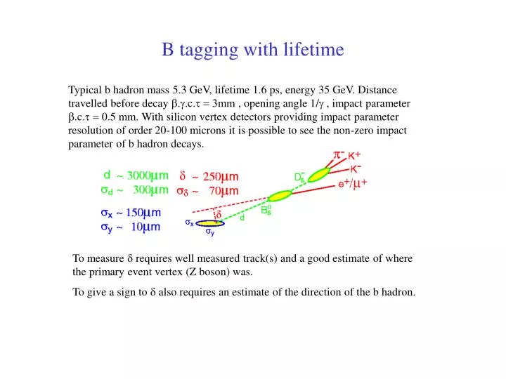
B tagging with lifetime Typical b hadron mass 5.3 GeV, lifetime 1.6 ps, energy 35 GeV. Distance travelled before decay b.g.c.t = 3mm , opening angle 1/g , impact parameter b.c.t = 0.5 mm. With silicon vertex detectors providing impact parameter resolution of order 20-100 microns it is possible to see the non-zero impact parameter of b hadron decays. To measure d requires well measured track(s) and a good estimate of where the primary event vertex (Z boson) was. To give a sign to d also requires an estimate of the direction of the b hadron.
Lifetime plot • This shows the distribution of the impact parameter significance, S, defined as the distance of closest approach to the primary vertex, divided by the uncertainty. S=d/sd. • The Monte Carlo is divided into three categories, b, c and uds. • Events with high S are mostly b • The background to the b events is mostly from charm • Large negative values of S are non-physical. They are due to badly reconstructed tracks and are independent of quark flavour.
Mass-lifetime tag Lifetime information is best used by constructing an overall confidence level that all the tracks in the hemisphere have S values consistent with zero. This is effective at distinguishing heavy from light flavours but it does not separate b from c. Use mass: B (d,b) is 4.2 GeV, D(c,u) is 1.9 GeV. Sort tracks in order of their S values. Starting with the highest S, successively add more tracks and calculate the combined invariant mass until it exceeds 1.8 GeV ( why not 1.9 GeV ? ). Take the S value of the last used track as a tag to distinguish b from c. Estimator based on lifetime alone. Estimator which combines lifetime and mass
b efficiency vs. background curve Having found a good discriminator between b jets and other jets, one can choose where to cut. Is it better to have high b efficiency and high backgrounds or low b efficiency and very low backgrounds ? In practice, carry out full analysis at several cut values and see which gives lowest total error. Aleph found optimum at 23% b efficiency and 0.6% c efficiency. Remember that b efficiency is measured with the data itself using the double tag method, so has little systematic error, whereas background is estimated with Monte Carlo simulation programs which are not perfect.
Identification of c jets In many respects c jets have properties somewhere intermediate between b jets and light (uds) jets. So they can be tagged but there are backgrounds to worry about on both sides. Also, decay of a b quark generally produces a c quark (Vcb ~ 0.04, Vub ~ 0.004). The c quarks coming directly from Z decay usually have higher momentum than those from the cascade Z b c. Who invented this naming system ? B mesons contain b quarks. D mesons contain c quarks. • c jets are identified by either • The semileptonic decay mode. Leptons with intermediate pl and pT in the jet, • Exclusive decay modes of D mesons, • Inclusive D* decay modes in which a characteristic very soft pion is found.
Exclusive (fully reconstructed) D decays Find tracks which are compatible with one of the known D decay modes and plot their invariant mass. Count events in the peak. Charge conjugation implied throughout. D*+p+D0 with D0 K- p+ or D0 K- p+p0or D0 K- p+ p- p+ D+ K- p+p+ D0 K- p+
Soft pions in D* decay The decay mode D*+(2010 MeV) p+ (140 MeV) D0 (1864 MeV) has very little energy available to give to the pion. The pion momentum in the D* rest frame is only 39 MeV, yet the branching ratio is 68%. c u The p+ will be boosted somewhat because the D* is moving in the jet direction. Even so, it will have low pL and very low pT with respect to the jet direction; even lower than most pions from hadronisation. This pion can be seen even if the D0 which goes with it is lost. c d u d This plot shows events where one jet was tagged with a D*+. The pT distribution of pions in the opposite jet is plotted. Z cc events will have soft pions of the opposite charge.
Partial width results All of the four LEP experiments have combined their partial width measurements together to produce these average results: for leptons Re = Ghadrons/ Gee etc. } Re = 20.804 ± 0.050 Rm = 20.785 ± 0.033 Rt = 20.764 ± 0.045 Lepton universality looks OK for hadrons Rb = Gbb/ Ghadrons etc. Rb = 0.21638 ± 0.00066 Rc = 0.1720 ± 0.0030 and the cross section at the peak for e– e+ Z hadrons: sh0 = 41.540 ± 0.0037 nb
Asymmetries at LEP1 and SLC • Three asymmetries could be measured at LEP1: • The forward-backward asymmetry, AFB, which is a measure of the angular distribution of the outgoing fermions from Z decay. Can be measured for each lepton type, for b and c quarks, and for all quark types averaged together. AFB = (sF - sB )/(sF + sB ) • The polarisation of the Z decay fermions. In practice this is only measurable in Z tt events, where the ts decay fast and their spin influences the momentum distribution of their decay products. Pt= (sPr - sPl )/(sPr + sPl ) • The variation of Pt with q. • Two more asymmetries could be measured at SLC because of the polarised beams. • The left-right asymmetry, ALR, which is a measure of the difference in the probability for producing Zs from left polarised electrons compared with right polarsied electrons. ALR = (sL - sR )/(sL + sR ). • The combined left-right forward-backward asymmetry which describes how the value of AFB depends on the polarisation of the incident electrons. ALRFB = (sLF+sRB-sLB-sRF)/ (sLF+sRB+sLB+sRF).
Asymmetries in the Standard Model Within the Standard Model at lowest order, all these asymmetries are determined by just one parameter; the weak mixing angle sin2qW. Small higher order corrections depend on particle masses. So precision measurement of the asymmetries provide a consistency test of the SM and can constrain the masses, mt and mH . The equations below give the relation between sin2qW and the asymmetries – for information, not to be memorsied! Vector and axial-vector coupling constants for each fermion type, f: gVf = I3f – 2.|Qf|. sin2qW , gAf = I3f , Af = 2. gVf .gAf / ( gVf 2 + gAf 2 ) where I3f is the isospin 3rd component: +½ if f = n or u-type quark, –½ if f = l– or d-type quark. Qf is the fermion charge. AFBf = ¾ .Ae.Af Pt = At Pt(q) = [At+2.Ae.cosq/(1+cos2q)]/[1+2.Ae. At cosq/(1+cos2q)] ALR = Ae ALRFB = ¾ Af