1 / 0

Chapter 8 The Classical Long-Run Model

CHAPTER. Chapter 8 The Classical Long-Run Model. Normative and Positive economics. Government borrowing increases interest rates The government role should be expanded in the economy. Economic Policy. Interesting and important question: - Does government spending financed

yagil
Download Presentation

Chapter 8 The Classical Long-Run Model

An Image/Link below is provided (as is) to download presentation Download Policy: Content on the Website is provided to you AS IS for your information and personal use and may not be sold / licensed / shared on other websites without getting consent from its author. Content is provided to you AS IS for your information and personal use only. Download presentation by click this link. While downloading, if for some reason you are not able to download a presentation, the publisher may have deleted the file from their server. During download, if you can't get a presentation, the file might be deleted by the publisher.

E N D

Presentation Transcript


  1. CHAPTER Chapter 8 The Classical Long-Run Model
  2. Normative and Positive economics. Government borrowing increases interest rates The government role should be expanded in the economy Economic Policy
  3. Interesting and important question: - Does government spending financed by borrowing improve the economy’s performance or make things worse? This has been debated for a long time and recently with the ARRA of 2009 - Its possible for both sides to be right. It depends on long-run vs short-run impact. Economic Policy
  4. Do the benefits of sort run impact out weight cost associated with long-run impact? We need to understand how the economy operated in the short-run and the long-run Chapter 8 addresses the long-run Economic Policy
  5. Macroeconomic Models Classical model Macroeconomic model that explains the long-run behavior of the economy We are talking about potential GDP. Look back at figures 4 and 5 in chapter 6. Developed by economists in the 19th and early 20th centuries The argued that market forces drive the economy toward full employment, possibly quickly.
  6. Potential Actual GDP Macroeconomics is concerned about both the trend and fluctuations around the trend Long-run real growth about 3% per year. Actual and Potential Real GDP, 1990–2011
  7. U.S. Real GDP, 1820–2010 (Logarithmic Scale) Classical economist certainly knew the economy fluctuated around the trend, but it always moved back on its own.
  8. Macroeconomic Models Great Depression Output was stuck far below its potential for many years 1936, John Maynard Keynes Keynesian model Classical model might explain the economy’s operation in the long run But, the long run could be a very long time in arriving Production could be stuck below its potential
  9. Macroeconomic Models Keynes’s ideas and further development help us understand economic fluctuations Movements in output around its long-run trend Quarter to quarter and year to year Classical model Has proven more useful in explaining the long-run trend itself Decades
  10. The Long-Run Classical Model Critical assumption about how the world works: Markets clear! The price in every market will adjust until quantity supplied and quantity demanded are equal Seems to be a reasonable assumption if trying to explain behavior of the economy over decades
  11. Classical Model We use the classical model to answer the following questions about the economy in the log-run: How is the level of total employment determined? How much output will we produce? What is the role of total spending in the economy? What happens when things change?
  12. How Much Output Will We Produce? Firms use resources (land, labor, capital and ______ to make the goods and services that people demand We’ll focus on labor and the labor market. We assume: Firms are already using the available quantities of the other resources Aggregate all the different types of labor into a single variable, labor
  13. The Labor Market Labor Supply and Demand Households (you and me) supply labor Firms demand labor Horizontal axis: number of workers Vertical axis: real hourly wage rate Real wage (we measure all variable in real terms) Measured in the dollars of some base year The amount of goods that workers can buy with an hour’s earnings
  14. The Labor Market Labor supply curve How many people will want to work at various real wage rates Slopes upward As the wage rate increases, more and more individuals decide they are better off working than not working
  15. The Labor Market Labor demand curve How many workers firms will want to hire at various real wage rates Downward sloping Firms maximize profits. As the wage rate decreases, each firm in the economy will find: To maximize profit, it should employ more workers than before When all firms behave this way together A decrease in the wage rate will increase the quantity of labor demanded in the economy
  16. Real Hourly Wage Excess Supply of Labor $30 LS H B A J E 25 150 million = Full Employment 20 Excess Demand for Labor LD Number of Workers Labor Market Equilibrium The equilibrium wage rate of $25 per hour is determined at point E, where the upward-sloping labor supply curve crosses the downward-sloping labor demand curve. At any other wage, an excess demand or excess supply of labor will cause an adjustment back to equilibrium.
  17. The Labor Market Equilibrium Equilibrium total employment Market clears In the Classical Model the economy achieves full employment on its own
  18. From Employment to Output Assumptions Quantities of other resources: fixed Technology: fixed Aggregate production function How much total output can be produced with different quantities of labor when quantities of all other resources and technology are held constant
  19. Aggregate production function Y output L labor
  20. Total Output (Real GDP) Real Hourly Wage In the labor market, the demand and supply curves intersect to determine employment of 150 million workers. The production function shows that those 150 million workers can produce $10 trillion of real GDP. LS $10 Trillion =Full Employment Output $25 150 million 150 million Number of Workers Number of Workers Aggregate Production Function LD Output Determination in the Classical Model
  21. From Employment to Output Equilibrium real GDP In the classical long-run view the economytends towards its potentialfull employment level of output on its own. http://www.cbo.gov/sites/default/files/cbofiles/attachments/Outlook%20Press%20Briefing%202013.pdf
  22. The Other Side of the MarketThe Role of Spending Total spending in a very simple economy, we assume: Households Spend all income on domestic output (no imports) No saving Domestic business firms No Government, no taxes. No exports or imports With these assumptions, total spending must be equal to total output
  23. An economy producing total output of $10 trillion will, by definition, create $10 trillion in factor payments or total income. If households spend all of this income on consumption goods, then total spending will equal $10 trillion as well. Total Spending in a Simple Economy
  24. The Role of Spending Say’s law (J.B. Say,1821) By producing goods and services (i.e., supply) firms create a total demand for goods and services equal to what they have produced Supply creates its own demand Full-employment can be maintained
  25. Total Spending in a More Realistic Economy Assumptions Still a closed economy (no imports or exports) But now have government Collects taxes and purchases goods and services Households No longer spend their entire income on consumption. Some is saved and they pay taxes Business firms Purchase capital goods (investment spending)
  26. Flows in the Economy of Classica, 2012
  27. Important definition;Planned investment spending (IP) IP=Business planned purchases of plant and equipment Total actual investment (I) = IP+Δinventories Δ inventories are treated as unplanned investment and can be positive or negative
  28. A couple of more definitions Net Taxes (T) Total government tax revenue minus government transfer payments Disposable income household income minus net taxes (Y – T) after tax income Household saving (S) - portion of after-tax income that households do not spend on consumption S= Disposable Income – C S = (Y - T - C)
  29. Household Saving (S) in our More Realistic Economy Household saving (S) S = (Y - T - C) = $10 - $1.25 - $7 = $1.75
  30. Total Spending in a More Realistic Economy Total spending in Classica Sum of the purchases made by Household sector (C) Business sector (IP) Government sector (G) Total spending = C + IP + G = $7 + $1 + $2 = $10
  31. More Important Stuff Leakages = T + S Income earned by households that they do not spend on the country’s output during a given year Injections = IP + G Spending on a country’s output from sources other than its households
  32. Even More Important Stuff At equilibrium, total output will equal total spending Y = C + IP + G And, at equilibrium, total leakages are equal to total injections S + T = IP + G Proof, from Y = C + IP + G we get, Y – C = IP+ G Y – C – T = IP + G –T (subtract T from each side) S = IP + G –T S + T = IP + G
  33. Leakages and Injections By definition, total output equals total income. Leakages: net taxes (T) and saving (S) - reduce consumption spending below total income. Injections: government purchases (G) plus planned investment spending (Ip) - contribute to total spending. When leakages equal injections, total spending equals total output.
  34. The Loanable Funds Market What guarantees that leakages are injected back into the spending stream? Answer: The loanable funds market Savers maker their funds available to borrowers Total supply of loanable funds is equal to household saving These funds are loaned out and households receive interest payments on these funds
  35. The Loanable Funds Market Supply of funds curve (saving) shows the level of household saving at various interest rates slopes upward: quantity of funds supplied to the financial market increases as the interest rate increases.
  36. Interest Rate Total Supply of Funds (Saving) 5% As the interest rate rises, saving or the quantity of loanable funds supplied increases B A 3% 1.75 1.5 Remember: As households save more they spend less Trillions of Dollars per Year Household Supply of Loanable Funds
  37. The Loanable Funds Market Demand for loanable funds isborrowing by business firms and government agencies Business demand for loanable funds is equal to their planned investment spending level of investment spending firms plan at various interest rates
  38. The Loanable Funds Market When the interest rate falls investment spending rises andbusiness borrowing rises
  39. Interest Rate 5% As the interest rate falls, business firms demand more loanable funds for investment projects. B A 3% 1.5 1.0 Planned Investment (Ip) (Business Demand for Funds) Trillions of Dollars per Year Business Demand for Loanable Funds
  40. Now the Government Budget deficit, G > T Excess of government purchases over net taxes (G>T). In our economy, G = $2.0 and T = $1.25. The deficit = $0.75 trillion. Government’s demand for loanable funds is equal to its budget deficit The government borrowsand pays interest on funds borrowed Budget surplus, T - G Excess of net taxes over government purchases (T>G)
  41. The Loanable Funds Market Government demand for funds curve Amount of government borrowing at various interest rates We assume this is independent of the interest rate
  42. The Loanable Funds Market Total demand for loanable funds curve Total amount of borrowing at various interest rates = [Ip+(G-T)] As the interest rate decreases Total quantity of funds demanded rises Quantity of funds demanded by business firms increases Quantity demanded by the government remains unchanged
  43. and the government's demand for loanable funds … Interest Rate Interest Rate Interest Rate gives us the economy's total demand for loanable funds at each interest rate. Summing business demand for loanable funds at each interest rate … Total Demand for Funds [Ip+(G-T)] Government Demand for Funds (G-T ) Business Demand for Funds (Ip) 5% 5% 5% (a) (b) (c) B B A A A B 3% 3% 3% 2.25 1.5 1.75 1.0 Trillions of dollars per year Trillions of dollars per year Trillions of dollars per year 0.75 The Demand for Loanable Funds
  44. Equilibrium in the Loanable Funds Market Interest rate will rise or fall until the quantities of funds supplied and demanded are equal What about Say’s law? It holds as long as the loanable funds market clears Total spending equals total output when all leakages are injected back into spending True even in a more realistic economy
  45. Interest Rate Total Supply of Funds (Saving) 5% E 1.75 Total Demand for Funds [Ip+(G-T)] Trillions of Dollars per Year Loanable Funds Market Equilibrium
  46. The loanable funds market clears. Total leakages will equal total injections. The leakage of net taxes goes to the government and is spent on government purchases. If the government is running a budget deficit, it will also borrow part of the leakage of household saving and spend that too. How the Loanable Funds Market Ensures That Total Spending = Total Output Any household saving left over will be borrowed by business firms and spent on capital. Thus, every dollar of leakages turns into spending by either government or private business firms.
  47. Say’s law with equations
  48. Fiscal Policy in the Classical Model:What happens when things change? Fiscal policy Change in government purchases or net taxes designed to change total output Demand-side effects Macroeconomic policy effects on total output that work through changes in total spending Classical model conclusion: Fiscal policy has no demand-side effects!
  49. An Increase in Government Purchases Increase in G without a change in T: the government must borrow the additional funds interest rate increases causing Decrease in planned investment spending Decrease in consumption spending (households save more - increase in savings) The result is the government purchases crowd out the spending of households (C) and businesses (Ip)
  50. Interest Rate Total Supply of Funds (Saving) 5% 7% G↑ = AH B F A H 2.25 1.75 2.05 C↓ IP↓ Ip+G2-T Ip+G1-T Trillions of Dollars per Year Crowding Out from an Increase in Government Purchases Beginning from equilibrium at point A, an increase in the budget deficit caused by additional government purchases shifts the demand for funds curve from Ip + G1 − T to Ip+ G2 − T. At point H, the quantity of funds demanded exceeds the quantity supplied, the interest rate begins to rise. As it rises, households save more, and business firms invest less. In the new equilibrium at point B, both consumption and investment spending have been completely crowded out by the increased government spending.
  51. Crowding Out Crowding out is the decline in one sector’s spending caused by an increase in some other sector’s spending Complete crowding out a dollar-for-dollar decline in one sector’s spending caused by an increase in some other sector’s spending What caused the crowding out????
  52. The Bottom Line In the classical model an increase in government purchases (G) Completely crowds out private sector spending Total spending remains unchanged No demand-side effects on total output or total employment
  53. A Decrease in Net Taxes Government cuts net taxes (T) Why? To increase total spending. Assume: households spend the entire tax cut Budget deficit increases Increase in government demand for funds Interest rate increase Decrease in planned investment spending Decrease in consumption spending as households save more
  54. Interest Rate T ↓ = AH = Initial C ↑ 5% 7% Total Supply of Funds (Saving) B F A H 2.25 1.75 2.05 C↓ Ip+G-T2 IP↓ Ip+G-T1 Trillions of Dollars per Year Crowding Out from a Tax Cut Beginning at point A, an increase in the budget deficit caused by a tax cut shifts the demand for funds curve from Ip + G − T1 to Ip + G − T2. If the tax cut is entirely spent, consumption initially rises by the distance AH. At the original interest rate of 5 percent, the quantity of funds demanded now exceeds the quantity supplied. This causes the interest rate to rise. As the interest rate rises, we move from A to B along the supply of funds curve. Saving rises (and consumption falls) by the distance AF. The final rise in consumption is FH. We also move along the demand for funds curve from H to B, so investment falls by the distance FH. In the new equilibrium at point B, consumption (which has risen by FH) has completely crowded out investment (which has dropped by FH).
  55. A Decrease in Net Taxes Bottom Line: In the classical a cut in taxes Raises consumption But interest rate increases which crowds out planned investment and consumption. Total spending remains unchanged No demand-side effects on total output or employment
  56. The Classical Model: A Summary Government Needn’t worry about employment The economy will achieve full employment on its own Needn’t worry about total spending The economy will generate just enough spending on its own to buy the output that a fully employed labor force produces Fiscal policy Has no demand-side effects on output or employment
More Related