Download
1 / 24
240 likes | 340 Views
Ocean Modeling Requirements for Decadal-to-Centennial Climate. Robert Hallberg NOAA/GFDL. Ocean Modeling Considerations for Decadal-Centennial Climate. Dec-Cen Climate is Operational, but not in Real Time. Ocean models are fully global and must include sea-ice.

E N D
Ocean Modeling Requirementsfor Decadal-to-Centennial Climate Robert Hallberg NOAA/GFDL
Ocean Modeling Considerationsfor Decadal-Centennial Climate • Dec-Cen Climate is Operational, but not in Real Time. • Ocean models are fully global and must include sea-ice. • Models run for O(1000-year) timescales. • Wall-clock model speeds are 103-104 times real time. • Ocean biases after a spinup of hundreds of years must be acceptably small. • Data assimilation during the run or unphysical damping are unacceptable in Dec-Cen climate models. • Precise initial values are often relatively unimportant. • The long timescales mean that a wide range of physical processes must be represented as credibly as possible.
Ocean Climate Models must be Conservative. • Non-conservation leads to drift and uncertainty. Tolerances for non-conservation: Mass – small compared to sea-level rise. 20th Century rise ~10 cm. Err << 10-3 m cen-1 ; MOM, GOLD ~10-7 m cen-1 Heat – small compared to anthropogenic forcing Anomalous Radiative Forcing ~4 W m-2 at CO2 doubling Err << 0.1 W m-2 ; MOM, GOLD ~3x10⁻⁶ W m-2 Total Salt – small compared to sea-level rise dilution? Dilution of Salinity ~ 10-3 PSU cen-1 Err << 10-4 PSU cen-1 ; MOM, GOLD ~3x10⁻⁹ PSU cen-1 With care, these tolerances can be achieved in all classes of ocean models. (MOM Z-coord., GOLD r-coord.)
Key Metrics of a Global Ocean Climate Model • SST biases at equilibrium • ENSO statistics (Amplitude & Frequency) at equilibrium • Tropical ocean circulation and watermass structure at equilibrium. • Stability and strength of meridional overturning circulation and gyre circulations. (Important for meridional heat transport & sea-ice distribution) • Equilibrium watermass properties, rates and processes of formation & destruction. (Important for storage of heat, carbon, etc.) • Spurious diapycnal mixing << physical – Kd = 10-5 to 10-6 m2 s-1 • Overflows & entraining gravity currents • Mode-water formation processes
100-year-mean SST Biases in GFDL’s CM2.1 Coupled Climate Model
Equatorial Pacific Velocities and Temperatures after 500 years in CORE simulations with 7 models Drifts accumulate over ~50 years. Short runs may not be indicative of equilibrium climate. (Figs. from Griffies et al., Ocean Mod., Sub.)
Challenges in Global Ocean Climate Modeling • Increasing resolution to admit mesoscale eddies
Role of eddies in Southern Ocean Dynamics • Eddies alter the sensitivity to forcing changes of the Southern Ocean overturning circulation and the resultant ventilation of the interior ocean. Hallberg & Gnanadesikan, JPO 2006
Challenges in Global Ocean Climate Modeling • Increasing resolution to admit mesoscale eddies • Dramatic increase in model cost, reduction in speed • Changes in required parameterizations • Numerical constraints (e.g. on spurious diapycnal mixing) become harder to satisfy. • Regional climate impacts
SST in a Prototype 1/8° Global Ocean Model Upwelling zone California Current ~1°×1° Box Contemporary Climate Model Resolution
Challenges in Global Ocean Climate Modeling • Increasing resolution to admit mesoscale eddies • Dramatic increase in model cost, reduction in speed • Changes in required parameterizations • Numerical constraints (e.g. on spurious diapycnal mixing) become harder to satisfy. • Regional climate impacts • Dominant scales of many ecosystems much smaller than well-resolved by global physical climate models. • Two-way nesting is probably needed.
ρ σ z z/z*/p/p* ROMS POM Poseidon HIM MITgcm MOM POP HyCOM The Existing GFDL Suite of Ocean Models • GFDL/Princeton has leading developers of each widely used class of large-scale ocean models. MOM – B-grid Z-coordinate model MITgcm – C-grid Z-coordinate model with nonhydrostatic capabilities HIM – C-grid isopycnal coordinate model POM – Princeton AOS program’s C-grid sigma coordinate model • The “Generalized Ocean Layer Dynamics” (GOLD) ocean model unites the GFDL efforts. GOLD is an ocean modeling system that combines the capabilities of GFDL’s MOM and HIM and the MITgcm ocean models into a single flexible code-base. GOLD numerics will be suitable for studying climate, but with demonstrated proficiency for a variety of other applications (tides, nonhydrostatic mixing, etc.) GOLD will include significant nesting and data assimilation capabilities. • GFDL ocean models focus on integrity for climate applications. Developers at GFDL/Princeton
GOLD and HYCOM • GOLD is structurally compatible with HYCOM. • The GOLD dynamic core & overall structure are derived from the isopycnal coordinate model HIM. Similar issues must be addressed as for HYCOM. • GOLD has necessary qualities for long-term climate studies. • Conservation-to-roundoff of heat, salt, mass, and tracers. • Accurate with a fully nonlinear equation of state. • Robust parameterizations of small-scale processes. • Rotated diffusion tensor & minimized spurious diapycnal mixing. • An NSF-funded project, including GOLD, HYCOM and ROMS, is exploring standardization across ocean models. • Collaborations are welcomed, provided they do not disrupt GFDL’s primary mission in long-term climate studies. GOLD ρ z z/z*/p/p* Poseidon HIM MITgcm MOM POP HyCOM
Potential for “One NOAA Ocean Model” Addressing Real-time Operational & Global Dec-Cen Climate What is a “model”? • A single model configuration. • Unlikely, due to mismatch in timescales, model speed, emphasis on initial conditions vs. bias. • A shared model code-base. • Repository of best theories/techniques for both real-time operations and climate. Natural synergies could emerge. • Will take considerable work and resources. • Important not to disrupt the on-going operational requirements for real-time forecasts or climate. • Establishing common model interfaces would be a natural first step. Some ocean forecasting applications (e.g., tsunami warnings) are so different that they are unlikely ever to use the same model.
High-Resolution Ocean Modeling &the Ocean Research Priorities Plan Numerical ocean models are recognized as crucial tools for a wide range of questions (ORPP, p. 47). • High resolution global ocean modeling is central to the ORPP’s Theme 4: “The Ocean’s Role in Climate” and the near-term priority “Assessing Meridional Overturning Circulation Variability” • Resolving the critical processes is crucial for reducing the uncertainty in projections. • The insight gained from the Global Ocean Observing System is maximized when the data is interpreted in the context of numerical models. • High resolution global ocean simulations are valuable in support of the other 5 Themes. • Provide consistent boundary conditions for ultrafine regional models. • Provide estimates of variability in the conditions faced by ecosystems, marine operations, or processes affecting human health. NOAA/GFDL is taking the lead in addressing the ORPP call for a coherent, comprehensive global modeling capability, addressing Theme 4 in particular.
34.7 Global Mean Ocean Salinity (PSU) CSM1 CSM2 GFDL1 GFDL2 Kiel MPI KNMI 34.6 0 200 300 400 500 100 Model Year Mean Salinity Drifts in 7 CORE Forced Candidate Ocean Climate models (Griffies et al., 2008) Notes: Sea-ice growth is the sole cause of salinity drift in some models. Some models balance salinity restoring, others do not.
Frontal Dynamics and Resolution • Upwelling jets & fronts require higher resolutions than current ocean climate models. • With steady forcing all variability is due to ocean dynamics. Hallberg & Gnanadesikan, JPO 2006
Strengths and Weaknesses of Terrain-following Coordinate Models (Issues for global climate application addressed in detail by G. Danabasoglu later.) Strengths: • Topography is represented very simply and accurately • Easy to enhance resolution near surface. • Lots of experience with atmospheric modeling to draw upon. Traditional Weaknesses: • Pressure gradient errors are a persistent problem. • Errors are reduced with better numerics (e.g., Shchepetkin & McWilliams, 2003) • Gentle slopes (smoothed topography) must be used for consistency • Traditional requirement for stability (Beckman & Haidvogel, 1993): • ROMS requirement (Shchepetkin, pers. comm): • Spurious diapycnal mixing due to advection may be very large. (Same issue as Z-coord.) • Diffusion tensors may be especially difficult to rotate into the neutral direction. • Strongly slopes require larger vertical stencil for the isoneutral-diffusion operator. Myth: Near bottom resolution can be arbitrarily enhanced. • Hydrostatic consistency imposes horizontal resolution-dependent constraints on near-bottom vertical resolution, with serious implications for the ability to represent overflows
Resolution requirements for avoiding numerical entrainment in descending gravity currents. Z-coordinate: Require that AND to avoid numerical entrainment. (Winton, et al., JPO 1998) Many suggested solutions for Z-coordinate models: • "Plumbing" parameterization of downslope flow: Beckman & Doscher (JPO 1997), Campin & Goose (Tellus 1999). • Adding a separate, resolved, terrain-following boundary layer: Gnanadesikan (~1998), Killworth & Edwards (JPO 1999),Song & Chao (JAOT 2000). • Add a nested high-resolution model in key locations? Sigma-coordinate:Avoiding entrainment requires that But hydrostatic consistency requires Isopycnal-coordinate:Numerical entrainment is not an issue - BUT • If resolution is inadequate, no entrainment can occur. Need
Maximum Hydrostatically Consistent Horizontal Resolution Horizontal Resolution (in km) Required to Permit 50m Vertical Resolution at Bottom
Maximum Hydrostatically Consistent Horizontal Resolution Horizontal Resolution (in km) Required to Permit 50m Vertical Resolution at Bottom
Maximum Hydrostatically Consistent Horizontal Resolution Horizontal Resolution (in km) Required to Permit 50m Vertical Resolution at Bottom