Download
1 / 1
10 likes | 122 Views
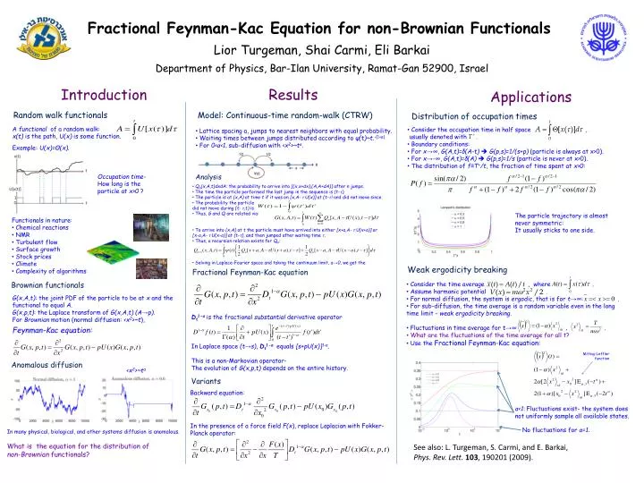
Fractional Feynman-Kac Equation for non-Brownian Functionals. Lior Turgeman, Shai Carmi, Eli Barkai. Department of Physics, Bar-Ilan University, Ramat-Gan 52900, Israel. Introduction. Results. Applications. Random walk functionals. Model: Continuous-time random-walk (CTRW).

E N D
Fractional Feynman-Kac Equation for non-Brownian Functionals Lior Turgeman, Shai Carmi, Eli Barkai Department of Physics, Bar-Ilan University, Ramat-Gan 52900, Israel Introduction Results Applications Random walk functionals Model: Continuous-time random-walk (CTRW) Distribution of occupation times • Consider the occupation time in half space , usually denoted with . • Boundary conditions: • For x→∞, G(A,t)=δ(A-t) G(p,s)=1/(s+p) (particle is always at x>0). • For x→-∞, G(A,t)=δ(A) G(p,s)=1/s (particle is never at x>0). • The distribution of f≡T+/t, the fraction of time spent at x>0: A functional of a random walk: x(t) is the path, U(x) is some function. • Lattice spacing a, jumps to nearest neighbors with equal probability. • Waiting times between jumps distributed according to ψ(t)~t.-(1+α) • For 0<α<1, sub-diffusion with <x2>~tα. Example: U(x)=Θ(x). Analysis Occupation time- How long is the particle at x>0 ? • Qn(x,A,t)dxdA: the probability to arrive into [(x,x+dx),(A,A+dA)] after n jumps. • The time the particle performed the last jump in the sequence is (t-τ). • The particle is at (x,A) at time t if it was on [x,A- τ U(x)] at (t-τ)and did not move since. • The probability the particle did not move during (t- τ,t) is • Thus, G and Q are related via: • To arrive into (x,A) at t the particle must have arrived into either [x+a,A- τ U(x+a)] or [x-a,A- τ U(x-a)] at (t-τ), and then jumped after waiting time τ. • Thus, a recursion relation exists for Qn: • Solving in Laplace-Fourier space and taking the continuum limit, a→0, we get the The particle trajectory is almost never symmetric: It usually sticks to one side. • Functionals in nature: • Chemical reactions • NMR • Turbulent flow • Surface growth • Stock prices • Climate • Complexity of algorithms Weak ergodicity breaking Fractional Feynman-Kac equation Brownianfunctionals • Consider the time average , where . • Assume harmonic potential . • For normal diffusion, the system is ergodic, that is for t→∞: . • For sub-diffusion, the time average is a random variable even in the long time limit - weak ergodicity breaking. • Fluctuations in time average for t→∞ , . • What are the fluctuations of the time average for all t? • Use the Fractional Feynman-Kac equation: G(x,A,t): the joint PDF of the particle to be at x and the functional to equal A. G(x,p,t): the Laplace transform of G(x,A,t)(A→p). For Brownian motion (normal diffusion: <x2>~t), Feynman-Kac equation: Dt1-α is the fractional substantialderivative operator In Laplace space (t→s), Dt1-α equals [s+pU(x)]1-α. This is a non-Markovian operator- The evolution of G(x,p,t) depends on the entire history. Mittag-Leffler function Anomalous diffusion <x2>~tα Variants Backward equation: α<1: Fluctuations exist- the system does not uniformly sample all available states. In the presence of a force field F(x), replace Laplacian with Fokker-Planck operator: No fluctuations for α=1. In many physical, biological, and other systems diffusion is anomalous. What is the equation for the distribution of non-Brownian functionals? See also: L. Turgeman, S. Carmi, and E. Barkai, Phys. Rev. Lett.103, 190201 (2009).