Download
1 / 111
1.3k likes | 2.38k Views
COE 341: Data & Computer Communications (T061) Dr. Radwan E. Abdel-Aal. Chapter 5: Signal Encoding Techniques. Where are we:. Chapter 7: Data Link: Flow and Error control. Data Link. Chapter 8: Improved utilization: Multiplexing. Physical Layer.

E N D
COE 341: Data & Computer Communications (T061)Dr. Radwan E. Abdel-Aal Chapter 5: Signal Encoding Techniques
Where are we: Chapter 7: Data Link: Flow and Error control Data Link Chapter 8: Improved utilization: Multiplexing Physical Layer Chapter 6: Data Communication: Synchronization, Error detection and correction Chapter 4: Transmission Media Transmission Medium Chapter 5: Encoding: From data to signals Chapter 3: Signals and their transmission over media, Impairments
Agenda • Overview: Implementation of the 4 encoding combinations introduced in chapter 3 • Encoding Digital Data as Digital Signals • Encoding Digital Data as Analog Signals • Encoding Analog Data as Digital Signals • Encoding Analog Data as Analog Signals
Four Data/Signal Combinations 4 3 2 1
Encoding Techniques 1. Digital data as digital signal 2. Digital data as analog signal: Converter (Modem) 3. Analog data as digital signal: Converter (Codec) 4. Analog data as analog signal • In general: • When the outcome is a digital signal we use an Encoding process • When the outcome is an analog signal we use a Modulation process • But we call the modulation of analog signal by digital datashift-keying
x(t) t s(f) f m(f) m(f) fc 0 0 Encoding: x(t) g(t) g(t) Encoder Decoder Analog Data Analog Data Digital Signal Transmission Modulation: Shift in frequency Shift back in frequency m(t) s(t) Demodulator Modulator m(t) Analog Data Analog Data Analog Signal Transmission fc fc Higher frequency Baseband Link Source Baseband Destination
Encoding and Modulation: Remarks • Encoding is simpler and less expensive than modulation • Encoding into digital signals allows use of modern digital transmission and switching equipment • Basis for Time Division Multiplexing (TDM) • Modulation shifts baseband signals to a higher region in the frequency spectrum (needs same fcs at both ends) • Basis for Frequency Division Multiplexing (FDM) • Optical fibers and unguided media and can carry only analog signals
Terminology • Unipolar Signals • Binary data represented by signals of the same polarity, e.g. 0: +5 V, 1: +10 V DC content • Bipolar (Polar) Signals • Binary data represented by signals of opposite polarity, e.g. 0: +5 V, 1: -5 V ideally Zero DC content
Terminology, Contd.Data rate and Signaling rate • Not always Tb = Ts !! • Multi-symbol transmission (M = 4, 8, …): Tb < Ts • Return to zero (RZ) codes: Ts < Tb • Mark and Space • Binary 1 and Binary 0 respectively • Duration of a bit (Tb) • Time taken for transmitter to emit a data bit • Data rate, R ( = 1/Tb) • Rate of data transmission • Measured in bits per second (bps) • Duration of a Signal Element (Ts) • Minimum duration of a signal pulse • Modulation (signaling) rate, D (1/Ts) • Rate at which the signal level changes with time • Measured inbauds = signal elements per second
Example: Two different coding methods Tb Data rate = 1/1ms = 1 M bps (in both cases) Signaling Rate for NRZI: = 1/1ms = 1 M bauds Signaling Rate for Manchester: = 1/0.5ms = 2 M bauds Ts Ts
Interpreting Received Signals • Requirements at RX: • Determine timing of bits – Bit start and end (When to look) Need Synchronization (Chapter 6) • Detect signal levels at mid-bit points • Compare signal level with a threshold level to decide on data • Factors affecting successful signal interpretation (Affect bit error rate) • Bandwidth • Signal to noise ratio • Data rate • Also Encoding/Modulation scheme, e.g. binary or multi-level
1. Digital Data, Digital Signal • Digital signal • Voltage/current pulses having a few discrete levels (2 levels for binary) • Each pulse is a signal element • Binary data is encoded into those signal elements
Encoding SchemesEncoding: Mapping data to signal elements Schemes for encoding digital data as digital signals • The Nonreturn to Zero (NRZ) Group: • Nonreturn to Zero-Level (NRZ-L) • Nonreturn to Zero Inverted (NRZI) • The Multi-level Binary Group: • Bipolar-AMI (Alternate Mark Invert) • Pseudoternary • The Bi-Phase (RZ) Group: • Manchester • Differential Manchester • Scrambling Group: • B8ZS (Bipolar with 8-Zeros Substitution) • HDB3 (High Density Bipolar 3-Zeros)
3 Power Spectral Density, Watt/Hz 1 2 4 1 1 0.5 1.5 0 Normalizedfrequency (f/r) Why so Many Encoding Schemes? Aspects of comparison between schemes: • Signal Spectrum: Desirable Features • Small high frequency content: Reduces effective bandwidth • No dc component: Allows ac transformer/capacitor coupling, required sometimes for electrical isolation • Concentrate signal power in the middle of the bandwidth: Avoids problems at BW edges, e.g. delay distortion. 2
Aspects of comparison between schemes: • Clocking Synchronizing RX to TX can be achieved using: • An external clock, or better: • A built-in synchronizing mechanism in the signal itself! (so, a code with many signal transitions is better) • Error detection • Mostly handled by higher layers, e.g. data link control • But error detection capabilities built into the signal encoding scheme would help! Advantage: Implemented much faster (in hardware)
Comparison of Encoding Schemes, contd. • Performance with interference and noise • Some encoding schemes perform better than others: e.g. with differential encoding: data is encoded as signal transition/no signal transition, and data detection at RX is less affected by noise • Cost and complexity • Some codes require signaling at a rate greater than the data rate (e.g. RZ) At higher signaling rates this requires higher bandwidth, faster circuits, etc. (larger costs)
3 1 2 4 1 1 0.5 1.5 0 NRZ GroupPros and Cons: • Pros • Easy to implement • Modest bandwidth requirements • Cons • Large DC component • Poor TX-RX synchronization: e.g. No signal transitions for long strings of all 0’s (so few edges are available for synchronization) • Used for magnetic recording • Not used much for signal transmission
The RZ Solution • Advantages of RZ: • Lower DC content (signal spends more time around 0V) • Guarantees an edge per bit (Better TX-RX synchronization) • Disadvantages of RZ: • Higher frequency content • More difficult to implement
NRZ Spectrum Power Spectral Density, Watt/Hz 1.5 B8ZS,HDB3 NRZ-L, NRZI 1 AMI, Pseudoternary 0.5 Mean square voltage per unit bandwidth Manchester, Differential Manchester 0 1 0.5 1.5 2 0 Frequency relative to data rate (binary data) -0.5 Normalizedfrequency (f/R)
NRZ-L: Non return to Zero-Level • Two different signal voltages for the 0 and 1 data bits • Voltage level is constant (no return to zero, so no signal transition) for the full duration of the data bit interval • e.g. 0 V for zero and a positive voltage for one • More often, negative voltage for one data value and positive for the other (bipolar signal) (Why?) • An example of absolute encoding: Mapping data directly to signallevels
NRZI: Nonreturn to Zero Invert • Still constant voltage level for bit duration of (hence NRZ) • But data is encoded as presence or absence of signal transition at the beginning of bit time: • Transition (low to high or high to low): Denotes binary 1 • No transition: Denotes binary 0 • This is an example of differential encoding: Encoding data as a change/no change in signal level
Differential Encoding • Data is represented by signal transitions rather than signal levels • Advantages; • With noise, signal transitions (or lack of them) are detected more easily than signal levels Better noise immunity • In complex transmission layouts, it is easy to accidentally lose sense of polarity RX • Effect of swapping terminals on: • NRZ-L • NRZI + _
The Multilevel Binary Group • Uses more than two signal levels (3 in this case) • Signal is multi-level but data is still binary! • Bipolar-AMI (Alternate Mark (1) Inversion) • 0 data is represented by no line signal • 1 data represented by positive or negative pulse • The “1” pulses alternate in polarity (why? 2 reasons!) • Advantages: • No net dc component (for any data sequence!) • Lower bandwidth than NRZ • No loss of sync with a long string of 1’z (but zeros still a problem- Will try to solve it later) • Alteration of pulse polarity also useful for error detection
Pseudoternary • Opposite of Bipolar-AMI: • 1 represented by no line signal • 0 represented by alternating positive and negative pulses • Could be called Bipolar-ASI: (Why?) • No advantage or disadvantage over bipolar-AMI
Signal Power density, Watt/Hz 1.5 B8ZS,HDB3 NRZ-L, NRZI 1 AMI, Pseudoternary 0.5 Mean square voltage per unit bandwidth Manchester, Differential Manchester 0 1 0.5 1.5 2 0 Frequency relative to data rate -0.5 Normalizedfrequency (f/r) Multilevel Spectrum
The Multilevel Binary Group: Advantages WK 9 • No net dc component • Spectrum centered at the middle of the BW • Lower bandwidth than NRZ • No loss of sync with a long string of 1’z (but zeros still a problem- Will try to solve it later) • Alteration of pulse polarity also useful for error detection: Next slide
Bipolar-AMI and Pseudoternary 1. All Single Pulse Errors- Detected 3. Double Pulse Error- Undetected Adding Canceling 2. Double Pulse Error- Detected
Disadvantages of Multilevel Binary N = Log2 (M) No. of bits sent during each signal element No. of signal levels used • Coding scheme not as efficient as NRZ: • We send only one bit at a time (1 or 0 data) Only M = 21 = 2 signal levels should be enough, but we are sending 3 levels > 2 ! • We use 3 signal levels Enough to represent log23 = 1.58 bits > 1 bit ! • Receiver Design and Noise Performance • Now receiver must distinguish between three signal levels (+A, -A, 0) Need better receiver design • Requires approximately 3dB higher SNR for the same probability of bit error (bit error rate)
Performance with noise: NRZ Vs AMI Multi-Level Binary (AMI) NRZ +A +A • For the same error rate: AMI requires higher SNR noise (lower noise) i.e. higher Eb/N0 (for same B and R) (hence the 3 dBs difference between the two curves) • For the same SNR (same Eb/N0 ) AMI has higher error rate • i.e. AMI has poorer performance with noise In both cases signal level is 2A pk2pk Noise level needed to cause an error 0 -A -A
The Biphase Group (2 signal phases per bit) • Manchester • Transition in middle of each bit period • Transition serves both as a clock edge and data representation • Low to high represents 1 • High to low represents 0 • Used by the IEEE 802.3 specification for Ethernet LAN (short distances) • Differential Manchester • Dedicated mid-bit transition used only for clocking • Data representation is at start of bit: • No transition at start of a bit period represents 1 • Transition at start of a bit period represents 0 (Inverts on 0’s – opposite of NRZI) • An example of differential encoding • Used by IEEE 802.5 specification for Token Ring LAN Examples of Self-Clocking Codes
Manchester Encoding • Mandatory transition in middle of each bit period • Low to high represents 1 • High to low represents 0 • Transitions at start of bit only where required Any error detection capabilities?? Note: This is not differential Data Representation Points
Differential Manchester Encoding • Mandatory midbit transition for clocking • Data represented by transition or no transition at bit start: • Transition (either direction)represents 0 • (Invert on zeros) • No transition represents 1 Any error detection capabilities?? Data Representation Points
Signal Power density, Watt/Hz 1.5 B8ZS,HDB3 NRZ-L, NRZI 1 AMI, Pseudoternary 0.5 Mean square voltage per unit bandwidth Manchester, Differential Manchester 0 1 0.5 1.5 2 0 Frequency relative to data rate -0.5 Normalizedfrequency (f/r) Biphase Group Spectrum Note higher frequency content
Biphase Pros and Cons • Pros • Guaranteed mid bit transitions • Synchronization facility (self clocking codes) • Ideally no dc component (using bipolar signals) • Error detection • Detecting absence of expected (mandatory) transitions • Cons • At least one transition per bit time and possibly two • Modulation (signaling) rate as high as twice that of NRZ • So, requires more bandwidth • Therefore, used over shorter distances (in LANs)
Tb Ts Data rate & Modulation (signaling) rate 3 bits TXed • Data rate, R = 1/Tbbps • Signaling Rate, D = 1/Tsbauds If we use k signal elements per bit, then: • Signaling (modulation) rate, D = Data rate, R (bit/s x k (signal elements/bit) Signal elements/s (bauds) Data Signal k=1 6 signal transitions = 6 signal elements Ts Ts Signal k=2 k = 6/3 = 2 • k = No. of signal elements/bit = No. of signal transitions (both ways)÷ No. of bits transmitted, n (over a given period of n Tbs)
Comparison of k for various encoding schemesat various data bit sequences k=2 e.g., here k = 1.5 i.e. baud rate D is 1.5 x data rate R
0 1 0 0 1 1 0 0 0 1 1 NRZ NRZI Manchester Differential Manchester Digital data, Digital signal Encoding Bipolar-AMI Pseudoternary Use plot to verify values of k in Table 5.3 on previous slide
Scrambling Group: B8ZS, HDB3Modifications on Bipolar Multilevel codes • Use bit scrambling to replace data bit sequences that would otherwise produce a constant signal voltage, with a more appropriate bit sequence producing signal changes • Helps overcome constant DC problems with Multilevel Binary codes (poor synch) • So, a “filling” (replacement) bit sequence is inserted where necessary • Criteria for a “Filling sequence” • Should produce enough transitions for synchronization • Must be recognized by receiver for replacement with original data • Not likely to be generated by noise (difficult for noise/interference to produce it) • Should occupy the same bit length as original data (so no extra overhead in the data rate)
Scrambling Group: B8ZS, HDB3 • Advantages: • No long sequences of zero level line signal • No dc component • No reduction in useful data rate (No extra data sent) • Built-in error detection capability
B8ZS • Bipolar With 8 Zeros Substitution • Improvement on bipolar-AMI • If an octet of 8 zeros and the last pulse preceding was positive (+):Transmitter encodes the 8 zeros as 000+-0-+ (how many level changes does this introduce?) • If an octet of 8 zeros and last voltage pulse preceding was negative (-): Transmitter encodes as 000-+0+- (shown in Fig. 5.6) • Each insertion has twointentional violations of the basic AMI code rule: (violations alternate in polarity- no net DC added) +000+-0-+ -000-+0+- • A strange event unlikely to be caused by noise • Receiver should detect it and interpret as an octet of 8 zeros (original data) • No additional data sent No penalty on genuine data rate
B8ZS -000-+0+- • See how the insertion satisfies the 5 requirements: • Detectable at RX • Difficult for noise to generate • Introduces transitions • Does not introduce DC (alternate violations) • Error detection capability V: Violation B: Bipolar (Valid)
HDB3 • High Density Bipolar 3 Zeros • Also based on bipolar-AMI • 4th zero always replaced with an intentional code violation • String of four zeros replaced with either: • 1 pulse -000- or +000+ (violation with preceding pulse) • or 2 pulses -+00+ or +-00- (internal violation within the insertion) • What determines whether 1 or 2 pulses? • Successive insertion violations must alternate in polarity (why?): -00000000 -000-+00+ or +00000000 +000+-00- • With insertions separated by n ‘1’ pulses: The new insertion is determined by the following rules (Table 5.4) • If n is even, with last pulse p (+ or -) p00p • If n is odd, with last pulse p (+ or -) 000p
HDB3 V: Violation B: Bipolar (Valid) -000-+00+ 1s Even number of 1s after last substitution, with the last pulse (+) p00p -00- Odd number of 1s after last substitution, with the last pulse (-) 000p 000- p p
Signal Power density, Watt/Hz 1.5 B8ZS,HDB3 NRZ-L, NRZI 1 AMI, Pseudoternary 0.5 Mean square voltage per unit bandwidth Manchester, Differential Manchester 0 1 0.5 1.5 2 0 Frequency relative to data rate -0.5 Normalizedfrequency (f/r) B8ZS, HDB3 Spectrum
2. Digital Data, Analog Signal Encoding • e.g. over public telephone system • 300Hz to 3400Hz • Use modem (modulator-demodulator) • Modulation (here called shift keying) manipulates one or more property of a carrier sine wave: • Amplitude shift keying (ASK) • Frequency shift keying (FSK) • Phase shift keying (PSK)
Modulation Techniques Digital Data Digital Signal Analog Signals FSK Phase shift angles = ? PSK
Amplitude Shift Keying (ASK) • Values represented by different amplitudes of the carrier sine wave • Usually, one amplitude is zero • i.e. presence and absence of carrier • e.g. switching the light sent through a fiber on and off • Susceptible to noise and sudden changes in gain • Up to 1200bps on voice grade lines • Used over optical fiber
Frequency Shift Keying (FSK) • Most common form is binary FSK (BFSK) • The two binary data values represented by two different frequencies (near and on both sides of a central carrier frequency fc) • Less susceptible to noise than ASK (Same as with FM Radio: Frequency can be detected correctly in the presence of noise better than amplitude) Applications: • Up to 1200bps on voice grade lines • Also used at High frequency radio (3-30 MHz) • And at even higher frequencies on LANs using coaxial cables Dfc Dfc f1 fc f2