Download
1 / 18
180 likes | 380 Views
1.2 - Investigating Polynomial Functions. MCB4U - Santowski. (A) Terminology. Polynomials : an expression in the form of a n x n + a n-1 x n-1 + a n-2 x n-2 + ...... + a 2 x² + a 1 x + a 0 where a 0 , a 1 , ...a n are real numbers and n is a natural number

E N D
1.2 - Investigating Polynomial Functions MCB4U - Santowski
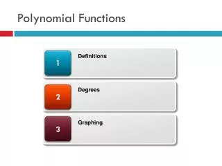
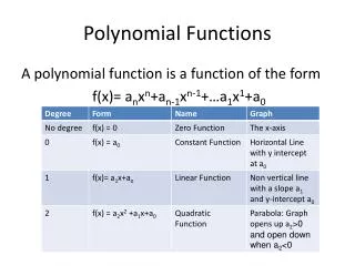
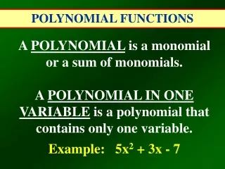
(A) Terminology • Polynomials: an expression in the form of anxn + an-1xn-1 + an-2xn-2 + ...... + a2x² + a1x + a0 where a0, a1, ...an are real numbers and n is a natural number • Polynomial Functions: a function whose equation is defined by a polynomial in one variable: • ex: f(x) = anxn + an-1xn-1 + an-2xn-2 + ...... + a2x² + a1x + a0 • leading coefficient: the coefficient of the term with the highest power • degree: the value of the highest exponent on the variable • Standard Form: the function is expressed such that the terms are written in descending order of the exponents
(A) Terminology • Domain: the set of all possible x values (independent variable) in a function • Range: the set of all possible function values (dependent variable, or y values) • to evaluate a function: substituting in a value for the variable and then determining a function value. Ex f(3) • finite differences: subtracting consecutive y values or subsequent y differences • zeroes, roots, x-intercepts: where the function crosses the x axes • y-intercepts: where the function crosses the y axes • direction of opening: in a quadratic, curve opens up or down • symmetry: whether the graph of the function has "halves" which are mirror images of each other
(A) Terminology • turning point: points where the direction of the function changes • maximum: the highest point on a function • minimum: the lowest point on a function • local vs absolute: a max can be a highest point in the entire domain (absolute) or only over a specified region within the domain (local). Likewise for a minimum. • increase: the part of the domain (the interval) where the function values are getting larger as the independent variable gets higher; if f(x1) < f(x2) when x1 < x2; the graph of the function is going up to the right (or down to the left) • decrease: the part of the domain (the interval) where the function values are getting smaller as the independent variable gets higher; if f(x1) > f(x2) when x1 < x2; the graph of the function is going up to the left (or down to the right) • "end behaviour": describing the function values (or appearance of the graph) as x values getting infinitely large positively or infinitely large negatively
(B) Types of Polynomial Functions • (i) Linear: Functions that generate graphs of straight lines, polynomials of degree one => f(x) = a1x1 + a0 or more commonly written as y = mx + b, or Ax + By + C = 0, or y = k(x - s) • (ii) Quadratic: Functions that generate graphs of parabolas; polynomials of degree two f(x) = a2x² + a1x1 + a0 or y = Ax² + Bx + C or y = a(x-s)(x-t) or y = a(x - h)² + k • (iii) Cubic polynomials of degree 3 • (iv) Quartic: polynomials of degree 4 • (v) Quintic: polynomials of degree 5
(C) Investigating Characteristics of Polynomial Functions • We can complete the following analysis for polynomials of degrees 1 through 5 and then make some generalizations or summaries: • In order to carry out this investigation, use either WINPLOT, a GDC • You may also use the following program from AnalyzeMath
(i) Linear functions • Determine the following for the linear functions • f(x) = 2x – 1 g(x) = -½x + 3 • (1) Leading coefficient (2) degree • (3) domain and range (4) evaluating f(-2) • (5) zeroes or roots (6) y-intercept • (7) Symmetry (8) turning points • (9) maximum values (local and absolute) • (10) minimum values (local and absolute) • (11) intervals of increase and intervals of decrease • (12) end behaviour (+x) and end behaviour (-x)
(ii) Quadratic Functions • For the quadratic functions, determine the following: • f(x) = x² - 4x – 5 f(x) = -½x² - 3x - 4.5 f(x) = 2x² - x + 4 • (1) Leading coefficient (2) degree • (3) domain and range (4) evaluating f(-2) • (5) zeroes or roots (6) y-intercept • (7) Symmetry (8) turning points • (9) maximum values (local and absolute) • (10) minimum values (local and absolute) • (11) intervals of increase and intervals of decrease • (12) end behaviour (+x) and end behaviour (-x)
(iii) Cubic Functions • For the cubic functions, determine the following: • f(x) = x3 - 5x² + 3x + 4 • f(x) =-2x3 + 8x² - 5x + 3 • f(x) = -3x3-15x² - 9x + 27 • (1) Leading coefficient (2) degree • (3) domain and range (4) evaluating f(-2) • (5) zeroes or roots (6) y-intercept • (7) Symmetry (8) turning points • (9) maximum values (local and absolute) • (10) minimum values (local and absolute) • (11) intervals of increase and intervals of decrease • (12) end behaviour (+x) and end behaviour (-x)
Conclusions for Cubic Functions • 1. Describe the general shape of a cubic function • 2. Describe how the graph of a cubic function with a positive leading coefficient is different than a cubic with a negative leading coefficient • 3. What does a0 represent on the graph of a cubic? • 4. How many real roots do/can cubic functions have? • 5. How many complex roots do/can cubic functions have? • 6. How many turning points do/can cubic functions have? • 7. How many intervals of increase do/can cubic functions have? • 8. How many intervals of decrease do/can cubic functions have? • 9. Describe the end behaviour (+x) of a cubic with a (i) positive (ii) negative leading coefficient • 10. Are cubic functions symmetrical? (You may need to investigate further)
(iv) Quartic Functions • For the quartic functions, determine the following: • f(x)= -2x4-4x3+3x²+6x+9 • f(x)= x4-3x3+3x²+8x+5 • f(x) = ½x4-2x3+x²+x+1 • (1) Leading coefficient (2) degree • (3) domain and range (4) evaluating f(-2) • (5) zeroes or roots (6) y-intercept • (7) Symmetry (8) turning points • (9) maximum values (local and absolute) • (10) minimum values (local and absolute) • (11) intervals of increase and intervals of decrease • (12) end behaviour (+x) and end behaviour (-x)
Conclusions for Quartic Functions • 1. Describe the general shape of a quartic function • 2. Describe how the graph of a quartic function with a positive leading coefficient is different than a quartic with a negative leading coefficient • 3. What does a0 represent on the graph of a quartic? • 4. How many real roots do/can quartic functions have? • 5. How many complex roots do/can quartic functions have? • 6. How many turning points do/can quartic functions have? • 7. How many intervals of increase do/can quartic functions have? • 8. How many intervals of decrease do/can quartic functions have? • 9. Describe the end behaviour (+x) of a quartic with a (i) positive (ii) negative leading coefficient • 10. Are quartic functions symmetrical? (You may need to investigate further)
(v) Quintic Functions • For the quintic functions, determine the following: • f(x)= x5+7x4-3x3-18x²-20 • f(x)= -¼x5+ 2x4-3x3+3x²+8x+5 • f(x)=(x²-1)(x²-4)(x+3) • (1) Leading coefficient (2) degree • (3) domain and range (4) evaluating f(-2) • (5) zeroes or roots (6) y-intercept • (7) Symmetry (8) turning points • (9) maximum values (local and absolute) • (10) minimum values (local and absolute) • (11) intervals of increase and intervals of decrease • (12) end behaviour (+x) and end behaviour (-x)
Conclusions for Quintic Functions • 1. Describe the general shape of a quintic function • 2. Describe how the graph of a quintic function with a positive leading coefficient is different than a quintic with a negative leading coefficient • 3. What does a0 represent on the graph of a quintic? • 4. How many real roots do/can quintic functions have? • 5. How many complex roots do/can quintic functions have? • 6. How many turning points do/can quintic functions have? • 7. How many intervals of increase do/can quintic functions have? • 8. How many intervals of decrease do/can quintic functions have? • 9. Describe the end behaviour (+x) of a quintic with a (i) positive (ii) negative leading coefficient • 10. Are quintic functions symmetrical? (You may need to investigate further)
(D) Examples of Algebraic Work with Polynomial Functions • ex 1. Expand & simplify h(x) = (x-1)(x+3)²(x+2). • ex 2. Where are the zeroes of h(x)? • ex 3. Predict the end behaviour of h(x). • ex 4. Predict the shape/appearance of h(x). • ex 5. Use a table of values to find additional points on h(x) and sketch a graph. • ex 6. Predict the intervals of increase and decrease for h(x). • ex 7. Estimate where the turning points of h(x) are. Are the max/min? and local/absolute if domain was [-4,1]
(D) Examples of Algebraic Work with Polynomial Funtions • ex 8. Sketch a graph of the polynomial function which has a degree of 4, a negative leading coefficient, 3 zeroes and 3 turning points • ex 9. Equation writing: Determine the equation of a cubic whose roots are -2, 3,4 and f(5) = 28 • ex 10. Prepare a table of differences for f(x) = -2x3 + 4x² - 3x - 2. What is the constant difference and when does it occur? Is there a relationship between the equation and the constant difference? Can you predict the constant difference for g(x) = 4x4 + x3 - x² + 4x - 5?
(E) Internet Links • Polynomial functions from The Math Page • Polynomial Functions from Calculus Quest • Polynomial Tutorial from WTAMU • Polynomial Functions from AnalyzeMath
(E) Homework • Nelson Text, page 14-17, Q1-3; zeroes and graphs 6,7; increase/decrease 9,10; equation writing11,14 • Nelson text page 23-26, Q1, end behaviour 5,6; combinations 7,8,9; graphs 11,12; finite differences 14,15