Download
1 / 44
500 likes | 860 Views
Chapter 6. Inputs and Production Functions. Chapter Six Overview. Motivation The Production Function Marginal and Average Products Isoquants The Marginal Rate of Technical Substitution Technical Progress Returns to Scale Some Special Functional Forms. Chapter Six.

E N D
Chapter 6 Inputs and Production Functions
Chapter Six Overview • Motivation • The Production Function • Marginal and Average Products • Isoquants • The Marginal Rate of Technical Substitution • Technical Progress • Returns to Scale • Some Special Functional Forms Chapter Six
Production of Semiconductor Chips • “Fabs” cost $1 to $2 billion to construct and are obsolete in 3 to 5 years • Must get fab design “right” • Choice: Robots or Humans? • Up-front investment in robotics vs. better chip yields and lower labor costs? • Capital-intensive or labor-intensive production process? Chapter Six
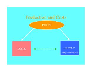
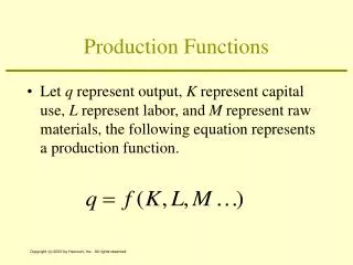
Key Concepts Productive resources, such as labor and capital equipment, that firms use to manufacture goods and services are called inputs or factors of production. The amount of goods and services produces by the firm is the firm’s output. Production transforms a set of inputs into a set of outputs Technology determines the quantity of output that is feasible to attain for a given set of inputs. Chapter Six
Key Concepts The production function tells us the maximum possible output that can be attained by the firm for any given quantity of inputs. • Production Function: • Q = output • K = Capital • L = Labor The production set is a set of technically feasible combinations of inputs and outputs. Chapter Six
The Production Function & Technical Efficiency Q Production Function Q = f(L) D • C • • B Production Set • A L Chapter Six
The Production Function & Technical Efficiency • Technically efficient: Sets of points in the production function that maximizes output given input (labor) • Technically inefficient: Sets of points that produces less output than possible for a given set of input (labor) Chapter Six
The Production Function & Technical Efficiency Chapter Six
Labor Requirements Function • Labor requirements function Example: for production function Chapter Six
The Production & Utility Functions Chapter Six
The Production & Utility Functions Chapter Six
The Production Function & Technical Efficiency Chapter Six
Total Product • Total Product Function: A single-input production function. It shows how total output depends on the level of the input • Increasing Marginal Returns to Labor: An increase in the quantity of labor increases total output at an increasing rate. • Diminishing Marginal Returns to Labor: An increase in the quantity of labor increases total output but at a decreasing rate. • Diminishing Total Returns to Labor: An increase in the quantity of labor decreases total output. Chapter Six
Total Product Chapter Six
The Marginal Product Definition: The marginal product of an input is the change in output that results from a small change in an input holding the levels of all other inputs constant. • MPL = Q/L • (holding constant all other inputs) • MPK = Q/K • (holding constant all other inputs) Example: Q = K1/2L1/2 MPL = (1/2)L-1/2K1/2 MPK = (1/2)K-1/2L1/2 Chapter Six
The Average Product & Diminishing Returns Definition: The average product of an input is equal to the total output that is to be produced divided by the quantity of the input that is used in its production: APL = Q/L APK = Q/K Example: APL = [K1/2L1/2]/L = K1/2L-1/2 APK = [K1/2L1/2]/K = L1/2K-1/2 Definition: The law of diminishing marginal returnsstates that marginal products (eventually) decline as the quantity used of a single input increases. Chapter Six
Total, Average, and Marginal Products Chapter Six
Total, Average, and Marginal Products Chapter Six
Total, Average, and Marginal Magnitudes TPL maximized where MPL is zero. TPL falls where MPL is negative; TPL rises where MPL is positive. Chapter Six
Production Functions with 2 Inputs • Marginal product: Change in total product holding other inputs fixed. Chapter Six
Isoquants Definition: An isoquanttraces out all the combinations of inputs (labor and capital) that allow that firm to produce the same quantity of output And… Chapter Six
Isoquants Chapter Six
Isoquants K Example: All combinations of (L,K) along the isoquant produce 20 units of output. Q = 20 Q = 10 Slope=K/L L 0 Chapter Six
Marginal Rate of Technical Substitution Definition: The marginal rate of technical substitutionmeasures the amount of an input, L, the firm would require in exchange for using a little less of another input, K, in order to just be able to produce the same output as before. MRTSL,K = -K/L (for a constant level of output) Marginal products and the MRTS are related: MPL(L) + MPK(K) = 0 => MPL/MPK = -K/L = MRTSL,K Chapter Six
Marginal Rate of Technical Substitution • The rate at which the quantity of capital that can be decreased for every unit of increase in the quantity of labor, holding the quantity of output constant, • Or • The rate at which the quantity of capital that can be increased for every unit of decrease in the quantity of labor, holding the quantity of output constant Therefore Chapter Six
Marginal Rate of Technical Substitution • If both marginal products are positive, the slope of the isoquant is negative. • If we have diminishing marginal returns, we also have a diminishing marginal rate of technical substitution - the marginal rate of technical substitution of labor for capital diminishes as the quantity of labor increases, along an isoquant – isoquants are convex to the origin. • For many production functions, marginal products eventually become negative. Why don't most graphs of Isoquants include the upwards-sloping portion? Chapter Six
Isoquants Isoquants K MPK < 0 Example: The Economic and the Uneconomic Regions of Production Q = 20 MPL < 0 Q = 10 L 0 Chapter Six
Marginal Rate of Technical Substitution Chapter Six
Elasticity of Substitution • A measure of how easy is it for a firm to substitute labor for capital. • It is the percentage change in the capital-labor ratio for every one percent change in the MRTSL,K along an isoquant. Chapter Six
Elasticity of Substitution Definition: The elasticity of substitution, , measures how the capital-labor ratio, K/L, changes relative to the change in the MRTSL,K. Chapter Six
Elasticity of Substitution • Example:Suppose that: • MRTSL,KA = 4, KA/LA = 4 • MRTSL,KB = 1, KB/LB = 1 • MRTSL,K = MRTSL,KB - MRTSL,KA = -3 • = [(K/L)/MRTSL,K]*[MRTSL,K/(K/L)] = (-3/-3)(4/4) = 1 Chapter Six
Elasticity of Substitution K "The shape of the isoquant indicates the degree of substitutability of the inputs…" = 0 = 1 = 5 = L 0 Chapter Six
Returns to Scale • How much will output increase when ALL inputs increase by a particular amount? Chapter Six
Returns to Scale Let λ represent the amount by which both inputs, labor and capital, increase. Let Φ represent the resulting proportionate increase in output, Q • Increasing returns: • Decreasing returns: • Constant Returns: Chapter Six
Returns to Scale • How much will output increase when ALL inputs increase by a particular amount? • RTS = [%Q]/[% (all inputs)] • If a 1% increase in all inputs results in a greater than 1% increase in output, then the production function exhibits increasing returns to scale. • If a 1% increase in all inputs results in exactly a 1% increase in output, then the production function exhibits constant returns to scale. • If a 1% increase in all inputs results in a less than 1% increase in output, then the production function exhibits decreasing returns to scale. Chapter Six
Returns to Scale K 2K Q = Q1 K Q = Q0 L 0 L 2L Chapter Six
Returns to Scale Chapter Six
Returns to Scale vs. Marginal Returns • Returns to scale: all inputs are increased simultaneously • Marginal Returns: Increase in the quantity of a single input holding all others constant. • The marginal product of a single factor may diminish while the returns to scale do not • Returns to scale need not be the same at different levels of production Chapter Six
Returns to Scale vs. Marginal Returns • Production function with CRTS but diminishing marginal returns to labor. Chapter Six
Technological Progress Definition:Technological progress (or invention) shifts the production function by allowing the firm to achieve more output from a given combination of inputs (or the same output with fewer inputs). Chapter Six
Technological Progress Labor saving technological progress results in a fall in the MRTSL,K along any ray from the origin Capital saving technological progress results in a rise in the MRTSL,K along any ray from the origin. Chapter Six
Neutral Technological Progress Technological progress that decreases the amounts of labor and capital needed to produce a given output. Affects MRTSK,L Chapter Six
Labor Saving Technological Progress • Technological progress that causes the marginal product of capital to increase relative to the marginal product of labor Chapter Six
Capital Saving Technological Progress Technological progress that causes the marginal product of labor to increase relative to the marginal product of capital Chapter Six