Matched Samples
Matched Samples. The paired t test. Sometimes in a statistical setting we will have information about the same person at different points in time.

Matched Samples
E N D
Presentation Transcript
Matched Samples The paired t test
Sometimes in a statistical setting we will have information about the same person at different points in time. A classical example of this is the pretest/posttest design (or the before and after test). The idea of this design is that we measure something (knowledge, weight, blood pressure, how much coke is enjoyed), then we do something to the person (educate them, have them do something, etc). After this intervention the subject is measured again. The point then is did the intervention somehow change the value of the measurement. (another application here is to have the same people do two things and measure after each and see if there is a difference.) It seems we have two populations to compare, the population before and the population after the intervention. In the context of having the same people involved at each point in time means we have a special design. We can do the matched sample inference methods.
Image you have data on people before and after some program. If for each person you calculate the value before minus after you will have a number for each person. In this sense we are right back to having a single variable. The inference procedures are right back to the population mean inference procedures for one variable. So, when we have matched samples two groups really collapses back to one group and the one variable is a difference in value variable. Another context would be that you do not have the same people, but the people in two groups have enough characteristics in common that you can consider them a matched sample. Then, again you calculate differences in the values and treat the differences as a single variable (instead of people you might have stores, or states or other units of analysis). In the context here we use a t statistic with df = n – 1. (It’s probably true the population standard deviation is unknown here.)
Since we are looking at hotels in the same cities at different times we really have a special case of statistical analysis. We can take the difference in the two time points. The difference is then a single variable. The population mean difference is denoted as μD and for ease of typing I will put this as muD. a) Here we have Ho: muD = 0 and H1: muD ≠ 0. This is a two tailed test with df = 17 and so we look in column .025 with alpha = .05. The critical t’s are -2.1098 and 2.1098. The tstat = (-78.68 – 0)/[48.611/sqrt(18)] = -78.68/11.46 = -6.87. Since the tstat is more extreme than the critical t’s we reject the null. We conclude the rates have changed!!!! c) Tail area for tstat = -6.87 is less than .005 and so the p-value < .01 and with alpha = .05 we reject the null.

