Statistical Inference

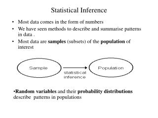
Statistical Inference • Most data comes in the form of numbers • We have seen methods to describe and summarise patterns in data . • Most data are samples (subsets) of the population of interest • Random variables and their probability distributions describe patterns in populations

Probability Distribution of a Discrete r.v. • The probabilities may be written as: • P(Xi=xi) is also referred to as the density function f(x) • The cumulative distribution function (c.d.f.) is defined as

X 1 2 . . . n f(x) 1/n 1/n 1/n 1/n 1/n 1/n Discrete Random Variables • 1 coin toss • 1 fair die throw • Examples of a discrete uniform distribution • We now look at non-uniform distributions

DISCRETE DISTRIBUTIONS Example - Family of 3 children. Let X be the Random Variable (RV) = number of girls Possible values: X = 3 GGG X = 2 GGB GBG BGG X = 1 BBG BGB GBB X = 0 BBB Assume the 8 outcomes are equally likely so that x 0 1 2 3 P(X = x) 1/8 3/8 3/8 1/8

Example - Bernoulli trials Each trial is an 'experiment' with exactly 2 possible outcomes, "success" and "failure" with probabilities p and 1-p. Let X = 1 if success, 0 if failure Probability distribution is x 0 1 P(X = x) p 1-p • Results for Bernoulli trials can be simulated using R • e.g. simulate results of a drug trial drug, success (cure) has probability p = 0.3 for each patient, 100 patients in trial. • result _ rbinom(100, size=1, prob=p) • result is a 100 vector that looks like 1,0,0,1,0,1,…...

Example-Binomial Experiment • Generalisation of Bernoulli trials • X ~ Bin(n,p)  X = # of successes in n Bernoulli trials • e.g. X = # of heads in 10 tosses of a coin, n = , p = • e.g. X = # of boys in a family of 5 children, n= , p = • e.g. X = # of sixes in 100 rolls of a dice, n= , p= • possible values for X = • probability distribution for X (q = 1-p) • P(X = k) Binomial expansion

Shape of the Binomial Distribution • The shape of the binomial distribution depends on the values of n and p. • probdistr_ dbinom(x=0:n, size=n, prob=p)

Expected Value of a Random Variable If the probability distribution of a random variable X is Values of X x1 x2 ... xk Probabilities p1 p2 ... pk its expected value is e.g. Drilling for oil Well Type Probability Pay-off Dry 0.5 0 Wet 0.4 $400K Gusher 0.1 $1500K

Expected values of drilling • Let random variable X be the financial gain • = pay-off - drilling cost • = pay-off - $200K • The probability distribution for X is • x -200 200 1300 • P(X=x) 0.5 0.4 0.1 • so the expected value (average) of X is • E(X) = -200 x 0.5 + 200 x 0.4 + 1300 x 0.1 = $110K • This is directly analogous to the sample mean • E(X) can be regarded as an idealisation of, or a theoretical value for, the sample mean • E(X) is often denoted by the Greek letter µ (pronounced "mu")

Variance of random variable • Recall that variance is a measure of spread. • For a sample the variance is • The variance of a r.v. X is : 2 =V(X) = E(X - )2 • 2 represents the theoretical limit of the sample variance s2 as the sample size n becomes very large. • A simpler formula for var(X) is 2 =V(X) = E(X2)- (E(X))2

Population equivalents of sample quantities Sample statistic Population parameter

Example - E(X) and V(X) • X = # of boys in a family of 5 children • X ~ Bin (5,0.5) • Then the probability distribution of X is x 0 1 2 3 4 5 P(X=x) 1/32 5/32 10/32 10/32 5/32 1/32 = np = npq

Transformations of random variables • If X is a r.v., then Y = 3X is also a r.v. Values of X x1 x2 ... xk Probabilities p1 p2 ... pk Values of Y 3x1 3x2 ... 3xk • In general, Y = f(X) is a r.v. with p.d.f. • fY(y)= P(Y=y) = P(X=f-1(y)) = fX(f-1(y)) • If X,Y are r.v.’s then Z = X + Y is also a r.v. • P.d.f. of Z is fZ(z) = fX*fY(z)

Example - 2 dice are thrown Let X denote the sum of the results. Outcomes: 11 21 31 41 51 61 12 22 32 42 52 62 13 23 33 43 53 63 14 24 34 44 54 64 15 25 35 45 55 65 16 26 36 46 56 66 Assume the 36 outcomes are equally likely so each has probability = 1/36 Possible values of X are 2, 3, ... , 12 e.g. P(X = 4) = P(1,3) + P(2,2) + P(3,1) = 3/36 . The probability distribution is x 2 3 4 . . . 10 11 12 P(X=x) 1/36 2/36 3/36 . . . 3/36 2/36 1/36

More E(X) and V(X) • If Y = a X + b , where X is a r.v. and a and b are known constant values, then E(Y) = a E(X) + b and V(Y) = a2V(X) (constant doesn’t count) • e.g. X = # boys in 5 children, Y = # girls in 5 children • Similarly if T = a X + b Y + c where X and Y are r.v. and a , b and c are known constants, then • E(T) = a E (X) + b E (Y) + c and • V(T) = a2V(X) + b2V(Y)+ 2ab Cov(X,Y) • In particular, if X and Y are independent then the covariance cov(X,Y) is zero

2 dice continued • X = sum of two dice thrown • X = Y + Z, • Y,Z i.i.d Unif (1:6) • E(Y) = E(Z) = 3.5 • V(Y) = V(Z) = E(Y2)-(E(Y))2 = 2.91 • E(Z) = E(X) + E(Y) = 7 • V(Z) = V(X) + V(Y) = 5.82

E(X) and V(X) for Binomial • Let X be Bernoulli, i.e. X~Bin(1,p) • E(X) = 1.p + 0.(1-p) = p • E(X2) = p • V(X) = E(X2) – (E(X))2 = p – p2 = pq • Now let X~Bin(n,p) • X = X1 + X2 + ….+ Xn , Xi i.i.d. Bernoulli • E(X) = E(X1) + E(X2) + ….+ E(Xn) = np • V(X) = V(X1) + V(X2) + ….+ V(Xn) = npq

Difference of r.v. s • A component is made by cutting a piece of metal to length X and then trimming it by amount Y. Both of these processes are somewhat imprecise. The net length is then T = X - Y. • This is of the form T = a X + b Y with a = 1 and b = -1 • so E(T) = a E (X) + b E (Y) = 1 E(X) + (-1)E(Y) = E(X) - E(Y) • V(T) = a2V(X) + (-b)2 V(Y) = V(X) + V(Y) • i.e. var(T) is greater than either var(X) or var(Y), even though T = X - Y, because both X and Y contribute to the variability in T.

Statistical Inference