Download
1 / 14
150 likes | 268 Views
Bayes Rule and Bayesian Networks. Presentation by: Ravikiran Gunale Y7159. Bayes Rule: If conditional probability of event A, given event B is known, How to determine conditional probability of event B, given event A.

E N D
Bayes Rule and Bayesian Networks Presentation by: RavikiranGunale Y7159
Bayes Rule: If conditional probability of event A, given event B is known, How to determine conditional probability of event B, given event A. P (A/B)= P(B/A)P(A)/P(B) • Provides a mathematical rule to explain how you should change your existing beliefs in the light of new evidence.
Propositional logic fully formalized. • Common situation in human reasoning : To perform inference from incomplete and uncertain knowledge. • Propositional logic fails in this situation. • Hence, Bayes Rule and Bayesian Networks
Bayesian Networks: Probabilistic graphic model that represents a set of random variables and their conditional dependencies via a directed acyclic graph. Car example directed graph. Fuel meter standing start Clean spark plug Fuel
G=(V,E) ,a directed acyclic graph. • X is a Bayesian network with respect to G if its joint probability density function can be written as a product of the individual density functions, conditional on their parent variables. • X is a Bayesian network with respect to G if it satisfies the local Markov property: each variable is conditionally independent of its non-descendants given its parent variables.
An Example P(fo)=0.15 P(U)=0.1 P(do/ fo U )=0.99 P(do/ fo not U)=0.9 P(do/ not fo U)=0.97 P(lo/fo)=0.6 P(do/ not fo not U)=0.3 P(lo/ not fo)=0.15 P(H/do)=0.7 P(H/not do)=0.01 Family out (fo) Unhealthy(U) Lights on(lo) Dog out(do) Hear bark(H)
Independence assumption: • If there are n random variables ,the complete distribution is specified by 2^n -1 joint probabilities. • n=5 . 2^n-1 =31 .But we needed only 10 values. If n=10 , we need 21 values. Where is this savings coming from? • Bayesian Networks have built in independence assumptions. Family out and hear bark example.
d-seperation path: • Let P be a trail from u to v. Then P is said to be d-separated by a set of nodes Z iff one of the following holds: • P contains a chain, i → m → j, such that the middle node m is in Z, • P contains a chain, i ← m ← j, such that the middle node m is in Z, • P contains a fork, i ← m → j, such that the middle node m is in Z, or • P contains a fork i → m ← j,such that middle m is not in Z and no descendant of m is in Z. • If u and v are not d-seperated then they are d- connected.
Consistent probabilities: Consider a system in which we have P(A/B)=0.7, P(B/A)=0.3, P(B)=0.5 Above values are inconsistent. Following property of Bayesian networks comes to rescue: If you specify probabilities of all the nodes given all parent combinations. • The numbers will be consistent. • The network will uniquely define a distribution.
Inference and learning: Parameter learning: Case1 :Complete Data Each data set is a configuration over all the variables in a network. To ensure that the parameters are learned independently, we make two assumptions: • Global independence • Local independence
Maximium likelihood estimation: Likelihood of M given D is L(M/D)=P(d/M), d belongs to D. M is the network, D the set of cases. Then we choose the parameter that maximizes the likelihood: a`= arg max L(Ma/D). Bayesian estimation: • MLE has drawbacks when using for sparse database. • For Bayesian estimation , start with a prior distribution and use data to update the distribution.
Incomplete Data: Some values may be missing , intentionally removed and in extreme case some variables may simply not be observable. Approximate techniques are used for parameter estimation.
Structure Learning: • In simple case, Bayesian network can be specified by expert and used for inference. • In other applications, network structure and parameters must be learned from data. X→Y→Z Type 1 and 2 represent same dependency X←Y→Z Type 3 can be uniquely identified. X→Y←Z • Systematically the skeleton of the underlying graph is determined • Then all arrows are oriented, whose directionality is dictated by the conditional independencies observed.
Applications: • Most common application is medical diagnosis. For e.g. PATHFINDER, a program to diagnose disease of the lymph node. • Modeling knowledge in computational biology, decision support system, bioinformatics ,image processing etc.