Download
1 / 16
160 likes | 286 Views
Environmental Boundary Tracking Using Multiple Autonomous Vehicles. Mayra Cisneros & Denise Lewis Mentor: Martin Short July 16, 2008. Project Details. Goal: Using autonomous vehicles, track the boundary of some gas released in Los Angeles. Boundary tracking One autonomous vehicle

E N D
Environmental Boundary Tracking Using Multiple Autonomous Vehicles Mayra Cisneros & Denise Lewis Mentor: Martin Short July 16, 2008
Project Details • Goal: Using autonomous vehicles, track the boundary of some gas released in Los Angeles. • Boundary tracking • One autonomous vehicle • Multiple autonomous vehicles • Images with noise • Moving boundary • Gas diffusion • Evolve concentration equation • Include obstacles like buildings in the simulation • Sensor networks
Input: angular velocity , tracking velocity v User selects a point on the image If the point is inside the boundary, d=1 Else, d=-1 Set =0 For a fixed number of iterations = +d* If a full circle is completed, v=2*v If the boundary is crossed d=-d update using angle correction Boundary Tracking Algorithm – One Autonomous Vehicle • x=x+v*cos • y=y+v*sin Gradient-Free Boundary Tracking Zhong Hu (Kemp-Bertozzi-Marthaler 2004)
Starting inside the boundary Starting outside the boundary Boundary Tracking With One Autonomous Vehicle
CUSUM Filters • If the image has noise, the algorithm fails to track the boundary. In order to use the algorithm we have to use CUSUM filters: and are the accumulation threshold, is the image, is the intensity at point , is the threshold for the image, and and are the “dead-zone” parameters. Gradient-Free Boundary Tracking Zhong Hu (Kemp-Bertozzi-Marthaler 2004)
Without CUSUM With CUSUM CUSUM Filters
Boundary Tracking Algorithm – Multiple Autonomous Vehicle • Similar to the algorithm for one autonomous vehicle • Additional input: number of robots • The user can select a point on the image or a starting point can be randomly generated • Instead of using a for loop, the algorithm runs until all the robots have stopped • A robot stops when it intersects the boundary track of any other robot including itself
18 robots, without noise 18 robots, with noise Boundary Tracking With Multiple Autonomous Vehicles
Gas Diffusion • Concentration equation: • D ~ 0.15 cm2/s • Evolving the concentration equation over time will produce a simulation of gas diffusing – initial concentration – time – diffusion coefficient – radius
Boundary Tracking Algorithm - Diffusion Simulation • Uses the boundary tracking algorithm for multiple robots • Additional input: maximum time T, size of time step dt • Given an image, the user selects starting points for the robots • While t T and the robots aren’t done tracking the boundary • Create an image of the diffusion simulation at the current time step, t • Plot the current position of all the robots along with all the previous positions on the new image • t=t+dt
Smart Sleeping Policies for Energy Efficient Tracking in Sensor Networks • Tracks a randomly moving object in a dense network of wireless sensors. • Sensor may be put in a sleep mode to conserve energy. • Therefore, energy saving can result in tracking errors. Goal: Build a simulation of the algorithm where the trade off is optimized.
Assumptions • Sensor has a limited range for detecting the object. • The network is sufficiently dense. • Central controller assign sleep times. • A sensor that is asleep cannot be communicated with or woken up prematurely . • Once the object leaves the network, it will not return. • Markov chain is used to describe an object whose statistics are known a priori.
Sleeping Policies To determine the best sleeping policy: • Partially observable Markov decision process (POMDP). There is two solutions: • Optimal and suboptimal solutions. Suboptimal solution perform better than a random sleeping time.
Future Work • Including obstacles like buildings in the diffusion simulation. • Smart Sleeping Policies simulation • Tracking a randomly moving object in a dense network of wireless sensors.