Download
1 / 80
820 likes | 1.06k Views
Experimental Nuclear Structure Part I. Filip G. Kondev kondev@anl.gov. Workshop on “Nuclear Structure and Decay Data: Theory and Evaluation”, Trieste, Italy February 20 th -March 3 rd , 2006. Outline. Lecture I: Experimental nuclear structure physics

E N D
Experimental Nuclear StructurePart I Filip G. Kondev kondev@anl.gov Workshop on “Nuclear Structure and Decay Data: Theory and Evaluation”, Trieste, Italy February 20th-March 3rd, 2006
Outline • Lecture I: Experimental nuclear structure physics • reactions used to populate excited nuclear states • techniques used to measure the lifetime of a nuclear state • Coulomb excitation, electronic, specific activity, indirect • techniques used to deduce Jp • ICC, angular distributions, DCO ratios etc. • Lecture II: Contemporary Nuclear Structure Physics at the Extreme • spectroscopy of nuclear K-Isomers • physics with large g-ray arrays • gamma-ray tracking – the future of the g-ray spectroscopy Have attempted to avoid formulas and jargon, and material covered by other lecturers – will give many examples
Plenty of information on the Web Some Useful Books “Handbook of nuclear spectroscopy”, J. Kantele,1995 “Radiation detection and measurements”, G.F. Knoll, 1989 “In-beam gamma-ray spectroscopy”, H. Morinaga and T. Yamazaki, 1976 “Gamma-ray and electron spectroscopy in Nuclear Physics”, H. Ejiri and M.J.A. de Voigt, 1989 “Techniques in Nuclear Structure Physics”, J.B.A. England, 1964 “Techniques for Nuclear and Particle Physics Experiments”, W.R. Leo, 1987 “Nuclear Spectroscopy and Reactions”, Ed. J. Cerny, Vol. A-C “Alpha-, Beta- and Gamma-ray Spectroscopy”, Ed. K. Siegbahn, 1965 “The Electromagnetic Interaction in Nuclear Spectroscopy”, Ed. W.D. Hamilton, 1975
Input from many colleagues C.J. Lister and I. Ahmad, Argonne National Laboratory, USA M.A. Riley, Florida State University, USA I.Y. Lee, Lawrence Berkeley National Laboratory, USA D. Radford, Oak Ridge National Laboratory, USA A. Heinz, Yale University, USA C. Svensson, University of Guelph, Canada G.D. Dracoulis and T. Kibedi, Australian National University, Australia J. Simpson, Daresbury Laboratory, UK E. Paul, University of Liverpool, UK P. Reagan, University of Surrey, UK and many others …
~3000 ~6000 nuclei are predicted to exist ~3000 the knowledge is very limited!
Introduction • The nucleus is one of nature’s most interesting quantal few-body systems • It brings together many types of behaviour, almost all of which are found in other systems • The major elementary excitations in nuclei can be associated with single-particle and collective modes. • While these modes can exist in isolation, it is the interaction between them that gives nuclear spectroscopy its rich diversity
The Nucleus is Unique! • Its uniqueness arises on the one hand because all forces of the nature are presented in the nucleus - strong, electromagnetic, weak, and even gravity if one considered condensed stellar objects as a huge number of nuclei held together by the gravitational attraction, in contrast to all other known physical objects. • On the other hand, the small number of nucleons leads to specific finite-system effects, where even a few particles can change the “face” of the whole system.
The Nucleus and other many-body systems • The physics of the nucleus is not completely secluded from the other many-body systems known in the nature. • A variety of nuclear properties can be described by the shell model, where nucleons move independently in their average potential, in close analogy with the atomic shell model. • The nucleus often behaves collectively, like a fluid - even a superfluid, in fact the smallest superfluid object known in the nature and there are close analogies both to condensed matter physics and to familiar macroscopic systems, such as the liquid drop.
So to summarize … NUCLEAR PHYSICS IS A BIG CHALLENGE(because of complicated forces, energy scale, and sizes involved) The challenge is to understand how nucleon-nucleon interactions build to create the mean field or how single-particle motions build collective effects like pairing, vibrations and shapes NUCLEAR PHYSICS IS IMPORTANT(intellectually, astrophysics, energy production, and security) THIS IS A GREAT TIME IN NUCLEAR PHYSICS(with new facilities just around the corner we have a chance to make major contributions to the knowledge - with advances in theory we have a great chance to understand it all - by compiling & evaluating data we have a chance to support various applications and to preserve the knowledge for future generations!)
To learn many of the secrets of the nucleus - we have to put it at extreme conditions and study how it survives such a stress!
Nuclear Reactions – very schematic! p t CN r a multi-step process • Gamma-ray induced • no Coulomb barrier • Neutron induced • low-spin states • no Coulomb barrier • Light charged particles, e.g. p, d, t, a • Coulomb barrier • low-spin states • Heavy Ions (1970 - ????) • high-spin phenomena • nuclei away from the line of stability
Reactions with Heavy Ions – Classical Picture R, Rt, Rp – half-density radii b – impact parameter INELASTIC SCATTERING DIRECT REACTIONS “SOFT” GRAZING COMPOUND NUCLEUS b<R=Rp+Rt Rp FUSION b Rt R “HARD” GRAZING FRAGMENTATION DEEP INELASTC REACTIONS DISTANT COLLISION ELASTIC SCATTERING COULOMB EXCITATION b>R E<Vc
Heavy Ions at the Coulomb barrier Many properties of the collision can be quite well estimated by just using conservation of momentum and energy. Ecm = Mt / (Mb + Mt) Elab Energy scale on which fusion starts is determined by Coulomb barrier,Vcb Vcb = (4pe)-1 ZbZte2 / R = 1.44 ZbZt / 1.16 [(Ab 1/3+At 1/3) + 2] MeV Lmax = 0.22 R [ m (Ecm – Vcb) ]1/2 Excitation energy is usually lowered by Q-value and K.E. of evaporated particles E*residue = Ecm + Q – K.E. Velocity of center-of-mass frame, which is ~ velocity of fused residues br2 = 2 Mbc2 Elab / [ (Mb + Mt)c2]2
Decay of the Compound Nucleus • In a typical HI fusion-evaporation reaction the final nucleus is often left with L~60-80 hbar and Ex~30-50 MeV • The excited nucleus cools off by emitting g-rays - their typical number is quite large, usually 30-40and the average energy is ~1-2 MeV – it is not a trivial task to detect all of them - the big advantage came with the large g-ray arrays
Channel Selection for g-ray spectroscopy Detection of Light Charged Particles (a,p,n) PLUS Efficient, flexible, powerful.....inexpensive. MINUS Count-rate limited, Contaminant (Carbon etc, isotopic impurities) makes absolute identification of new nuclei difficult.CROSS SECTION LOWER LIMIT ~100 mb that is, ~10-4 Detection of Residues in Vacuum Mass Separator PLUS True M/q, even true M measurement. With suitable focal plane detector can be ULTRA sensitive. Suppresses contaminants. MINUS Low EfficiencyCROSS SECTION LOWER LIMIT ~100 nb that is ~10-7 Detection of Residues in Gas Filled Separator Improves efficiency of vacuum separators, at cost of mass information and cleanliness. In some cases (heavy nuclei) focal plane counters clean up the data for good sensitivity.
Some Channel Selection Detectors Argonne FMA USA Light charged-particle detector Microball – 96 CsI with photo diodes Jyvaskyla RITU USA Europe
Calculate Reaction Rates • Reaction Yield/sec. Y = Nb Nts • Nb = ib/e qwith ib = electric current in amps, q = charge state, e = 1.6 10-19 c • Nt = [Na /A] rxwith Na = Avagadros #, A = Mass # of tgt, r= density in g/cc, x = thickness (cm). • = Cross Section in cm2 .... note 1 barn is 10-24 cmAccumulated data: D = Y x TIME x Efficiency Typical not “far from stability” experiment may have:ib = 100 nA, q=10, A=100, rx= 10-3 & s=1 barn - produces 3x10⁵ reactions/sec BUT If partial cross section is 100 nb and efficiency is 10%...... rate is 10 /hour, 10 pb gives~ 1 every 10 weeks!!!.....the present situation for producing the heavies elements.
T1/2,es Ex Jp,K Eg T1/2,gs 0 0 Jp,K The basic knowledge What we want to know excited state • Excitation energy • Quantum numbers and their projections • Lifetime • Branching ratios a,b-,b+, EC,p, fission, g, ICC ground state stable or, a, b-, b+, EC, p, cluster, fission How • By measuring properties of signature radiations
What is Stable? • A surprisingly difficult question with a somewhat arbitrary answer!CAN’T Decay to something else, BUT • CAN’T Decay is a Philosophical Issue • Violation of some quantity which we believe is conserved such as Energy, Spin, Parity, Charge, Baryon or Lepton number, etc. • DOESN’T Decay is an Experimental Issue that backs up the beliefs Specific Activity: A=dN/dt = lN Activity of 1 mole of material (6.02 x 10²³ atoms) with T1/2=109 y (l=2.2 x 10⁻¹⁷ s) is ~0.4 mCi (1 Ci=3.7 x 10¹⁰ dps) (or 13 MBq) .... a blazing source, so it is quite easy to set VERY long limits on stability. Current limit on proton half-life, based on just counting a tank of water is T1/2> 1.5 x 1025 yr.
Stable Nuclei: Segre’s Chart ~ 280 Nuclei have Half-lives >106 years So are (quite) stable against Decay of their constituents (p,n,e) Weak Decay (b+b– and E.C.) a,p,n decays More complex cluster emission Fission (Mostly because of energy conservation) N Atomic Number, Z
Mean Lifetime Probability for decay of a nuclear state (normalized distribution function); l - decay constant Probability that a nucleus will decay within time t Probability that a nucleus will remain at time t The average survival time (mean lifetime - t) is then the mean value of this probability
T1/2: the time required for half the atoms in a radioactive substance to disintegrate [eV] Half-life & Decay Width relation between t,T1/2 and l Determine the matrix element describing the mode of decay between the initial and final state
log ft values partial half-life of a given b-(b+,EC) decay branch statistical rate function (phase-space factor): the energy & nuclear structure dependences of the decay transition N.B. Gove and M. Martin, Nuclear Data Tables 10 (1971) 205
M.A. Preston, Phys. Rev. 71 (1947) 865 I. Ahmad et al., Phys. Rev. C68 (2003) 044306 Hindrance Factor in a-decay Strong dependence on L L=0 - unhindered decay (fast)
g-ray decay magnetic multipole electric multipole octupole hexadecapole quadrupole dipole
Partial lifetime & Transition Probability partial half-life partial g-rayTransition Probability reducedTransition Probability contains the nuclear structure information
Hindrance Factor in g-ray decay Hindrance Factor:Weisskopf (W): based on spherical shell model potential Nilsson (N): based on deformed Nilsson model potential … usually an upper limit, but …
10+ I 8+ 6+ 4+ 2+ 0+ I=Jw 156Dy Quadrupole Deformation 12+ deformed nucleus (from collective models) EI=h2/2J I(I+1) B(E2) ~ 200 W.U.
w W2 W1 K=W1+W2 K-forbidden decay Deformed, axially symmetric nuclei K is approximately a good quantum number each state has not onlyJp but also K • The solid line shows the dependence of FW on ΔK for some E1 transitions according to an empirical rule: log FW = 2{|ΔK| - λ} = 2ν • i.e. FW values increase approximately by a factor of 100 per degree of K forbiddenness • fn=(Fw)1/n – reduced hindrance per degree of K forbiddenness
Experimental techniques • Direct width measurements • Inelastic electron scattering • Blocking technique • Mossbauer technique
Time Range: a few seconds up to several years Specific Activity • Statistical uncertainties are usually small • Systematic uncertainties (dead time, geometry, etc.) dominate usually want to follow at least 5 x T1/2 Tag on specific signature radiations (a, b, ce or g) in a “singles” mode Clock Detector Source
Specific Activity: Example 1 • More than 270 spectra were measured • Followed 4 x T1/2 191.4
Specific Activity: Example 2 Si det C foil 1 GeV pulsed proton beam on 51 g/cm2 ThCx target on-line mass separation (ISOLDE)/CERN H. De Witte et al., EPJ A23 (2005) 243
Very long-lived cases – Example 1 Time Range: longer than 102 yr the number of atoms estimated by other means, e.g.mass spectrometry
a a a 250Cf 246Cm 242Pu 13 y 4747 y 5105 y Very long-lived cases – Example 2 parent daughter T1/2(250Cf)=13.05 (9) y • mass-separated source • alpha-decay counting technique T1/2 = 4747 (46) years / Compared to values ranging from T1/2=2300 up to 6620 years
Time Range: tens of ps up to a few seconds t Electronic techniques The “Clock” - TAC, TDC (START/STOP); Digital Clock t START START “singles” – Eg-time, Ea-time “coincidence” – Eg1-Eg2-Dt ; Ea1-Eg1-Dt Ea1-Ea2-Dt Difficulties at the boundaries: e.g. for very short– and very long-lived cases!
Prompt Response Function • all detectors and auxiliary electronics show statistical fluctuations in the time necessary to develop an appropriate pulse for the “clock” • depend on the characteristics of the detectors: e.g. light output for scintillators, bias voltage, detector geometry, etc. • instrumental imperfections in the electronics – e.g. noise in the preamplifiers Some typical values
Prompt Response Function: Ge detectors decay PRF a schematic illustration • PRF depends on: • the size of the detector • the energy of the g-ray
the shortest lifetime that can be measured is limited by the TOF Recoil-shadow technique thin production target
One example: 140Dy experiment at ANL 54Fe + 92Mo @ 245 MeV a2n channel, mass 140 only 5% from the total CS
Some of the equipments used … 1 70% Gammasphere HpGe detector 4 25% Golf-club style HPGe detectors 2 LEPS detectors 1 2"x2" Large Area Si detector 2"x2" Si Detector
T1/2=7.3 (15) ms 140Dy: Experimental Results Similar results by the ORNL group, Krolas et al., PRC 65, 2002 D.M. Cullen et al., Phys. Lett. B529 (2002)
The Heart of RDT: the DSSD 208Pb(48Ca,2n)254No 80 x 80 detector 300 mm strips,Each with high, low, and delay line amplifiers, for implant, decay, and fast-decay recognition. Data from DSSD showing implant pattern 40 cm beyond the focal plane
Timescale of Events Energy (MeV) a1: 6.12 MeV a2: 5.7 MeV T1st decay T2nd decay 0 Time 177Au Implant a-a (parent-daughter) correlations Implantation->Decay 1->Decay 2 within a single pixel F.G. Kondev et al. Phys. Lett. B528 (2002) 221