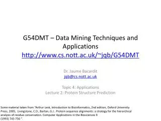
G54DMT – Data Mining Techniques and Applications cs.nott.ac.uk/~jqb/G54DMT

1. G54DMT – Data Mining Techniques and Applicationshttp://www.cs.nott.ac.uk/~jqb/G54DMT Dr. Jaume Bacardit jqb@cs.nott.ac.uk Topic 4: Applications Lecture 2: Protein Structure Prediction Some material taken from “Arthur Lesk, Introduction to Bioinformatics, 2nd edition, Oxford University Press, 2005, Livingstone, C.D., Barton, G.J.: Protein sequence alignments: a strategy for the hierarchical analysis of residue conservation. Computer Applications in the Biosciences 9 (1993) 745-756 ”.

2. Outline • Brief introduction to protein structure • Motivation and definition of PSP • PSP: A family of problems • Data Mining protein’s structural aspects • Dimensionality reduction for protein datasets • Summary

3. Protein Structure: Introduction • Proteins are molecules of primary importance for the functioning of life • Structural Proteins (collagen nails hair etc.) • Enzymes • Transmembrane proteins • Proteins are polypeptide chains constructed by joining a certain kind of peptides amino acids in a linear way • The chain of amino acids however folds to create very complex 3D structures • There is a general consensus that the end state of the folding process depends on the amino acid composition of the chain

4. Protein Structure

5. Amino Acids

6. Protein Structure: Introduction • Different amino acids have different properties • These properties will affect the protein structure and function • Hydrophobicity, for instance, is the main driving force (but not the only one) of the folding process

7. Global Interactions Local Interactions Protein Structure: Hierarchical nature of protein structure Primary Structure = Sequence of amino acids MKYNNHDKIRDFIIIEAYMFRFKKKVKPEVDMTIKEFILLTYLFHQQENTLPFKKIVSDLCYKQSDLVQHIKVLVKHSYISKVRSKIDERNTYISISEEQREKIAERVTLFDQIIKQFNLADQSESQMIPKDSKEFLNLMMYTMYFKNIIKKHLTLSFVEFTILAIITSQNKNIVLLKDLIETIHHKYPQTVRALNNLKKQGYLIKERSTEDERKILIHMDDAQQDHAEQLLAQVNQLLADKDHLHLVFE Secondary Structure Tertiary

8. Motivation for PSP • The function of a protein depends greatly on its structure • The structure that a protein adopts is vital to it’s chemistry • Its structure determines which of its amino acids are exposed to carry out the protein’s function • Its structure also determines what substrates it can react with • However the structure of a protein is very difficult to determine experimentally and in some cases almost impossible

9. Protein Structure Prediction • That is why we have to predict it • PSP aims to predict the 3D structure of a protein based on its primary sequence

10. Impact of PSP • PSP is an open problem. The 3D structure depends on many variables • It has been one of the main holy grails of computational biology for many decades • Impact of having better protein structure models are countless • Genetic therapy • Synthesis of drugs for incurable diseases • Improved crops • Environmental remediation

11. Prediction types of PSP • There are several kinds of prediction problems within the scope of PSP • The main one of course is to predict the 3D coordinates of all atoms of a protein (or at least the backbone) based on its primary sequence • There are many structural properties of individual residues within a protein that can be predicted for instance: • The secondary structure state of the residue • If a residue is buried in the core of the protein or exposed in the surface • Accurate predictions of these sub-problems can simplify the general 3D PSP problem

12. Prediction types of PSP • There is an important distinction between the two classes of prediction • The 3D PSP is generally treated as an optimisation problem • The prediction of structural aspects of protein residues are generally treated as machine learning problems

13. DATA MINING PROTEIN’S STRUCTURAL ASPECTS

14. Prediction of structural aspects of protein residues • Many of these features are due to local interactions of an amino acid and its immediate neighbours • Can it be predicted using information from the closest neighbours in the chain? • In this simplified example to predict the SS state of residue i we would use information from residues i-1 i and i+1. That is a window of ±1 residues around the target Ri-5 SSi-5 Ri-4 SSi-4 Ri-3 SSi-3 Ri-2 SSi-2 Ri-1 SSi-1 Ri SSi Ri+2 SSi+2 Ri+3 SSi+3 Ri+4 SSi+4 Ri+5 SSi+5 Ri+1 SSi+1 Ri-1 Ri Ri+1 SSi Ri Ri+1 Ri+2 SSi+1 Ri+1 Ri+2 Ri+3  SSi+2

15. ARFF file for a simple PSP dataset @relation AA+CN_Q2 @attribute AA_-4 {A,C,D,E,F,G,H,I,K,L,M,N,P,Q,R,S,T,V,W,X,Y} @attribute AA_-3 {A,C,D,E,F,G,H,I,K,L,M,N,P,Q,R,S,T,V,W,X,Y} @attribute AA_-2 {A,C,D,E,F,G,H,I,K,L,M,N,P,Q,R,S,T,V,W,X,Y} @attribute AA_-1 {A,C,D,E,F,G,H,I,K,L,M,N,P,Q,R,S,T,V,W,X,Y} @attribute AA {A,C,D,E,F,G,H,I,K,L,M,N,P,Q,R,S,T,V,W,Y} @attribute AA_1 {A,C,D,E,F,G,H,I,K,L,M,N,P,Q,R,S,T,V,W,X,Y} @attribute AA_2 {A,C,D,E,F,G,H,I,K,L,M,N,P,Q,R,S,T,V,W,X,Y} @attribute AA_3 {A,C,D,E,F,G,H,I,K,L,M,N,P,Q,R,S,T,V,W,X,Y} @attribute AA_4 {A,C,D,E,F,G,H,I,K,L,M,N,P,Q,R,S,T,V,W,X,Y} @attribute class {0,1} @data X,X,X,X,A,E,I,K,H,0 X,X,X,A,E,I,K,H,Y,0 X,X,A,E,I,K,H,Y,Q,0 X,A,E,I,K,H,Y,Q,F,0 A,E,I,K,H,Y,Q,F,N,0 E,I,K,H,Y,Q,F,N,V,0 I,K,H,Y,Q,F,N,V,V,0 K,H,Y,Q,F,N,V,V,M,1 H,Y,Q,F,N,V,V,M,T,0 Y,Q,F,N,V,V,M,T,C,1

16. What information do we include for each residue? • Early prediction methods used just the primary sequence  the AA types of the residues in the window • However the primary sequence has limited amount of information • It does not contain any evolutionary information it does not say which residues are conserved and which are not • Where can we obtain this information? • Position-Specific Scoring Matrices which is a product of a Multiple Sequence Alignment

17. Position-Specific Scoring Matrices (PSSM) • For each residue in the query sequence compute the distribution of amino acids of the corresponding residues in all aligned sequences (discarding those too similar to the query) • This distributions will tell us which mutations are likely and which mutations are less likely for each residue in the query sequence • In essence it’s similar to a substitution matrix but tailored for the sequence that we are aligning • A PSSM profile will also tell us which residues are more conserved and which residues are more subject to insertions or deletions

18. PSSM for the 10 first residues of 1n7lA A R N D C Q E G H I L K M F P S T W Y V A: 4 -1 -2 -2 0 -1 -1 0 -2 -1 -2 -1 -1 -2 -1 1 0 -3 -2 0 M:-1 -2 -3 -4 -2 -1 -2 -3 -2 1 2 -2 7 0 -3 -2 -1 -2 -1 1 E:-1 0 0 2 -4 2 6 -2 0 -4 -3 1 -2 -4 -1 0 -1 -3 -2 -3 K:-1 2 0 -1 -4 1 1 -2 -1 -3 -3 5 -2 -4 -1 0 -1 -3 -2 -3 V: 0 -3 -3 -4 -1 -3 -3 -4 -4 3 1 -3 1 -1 -3 -2 0 -3 -1 5 Q:-1 1 0 0 -3 6 2 -2 0 -3 -3 1 -1 -4 -2 0 -1 -2 -2 -3 Y:-2 -1 -1 -3 -3 -1 -1 -3 6 -2 -2 -2 -1 2 -3 -2 -2 1 7 -2 L:-2 -3 -4 -4 -2 -3 -3 -4 -3 2 5 -3 2 0 -3 -3 -1 -2 -1 1 T: 0 -1 0 -1 -1 -1 -1 -2 -2 -1 -1 -1 -1 -2 -1 2 5 -3 -2 0 R:-2 6 -1 -2 -4 1 0 -3 0 -3 -3 2 -2 -3 -2 -1 -1 -3 -2 -3

19. Secondary Structure Prediction • The most usual way is to predict whether a residue belongs to an α helix a β sheet or is in coil state • Several programs can determine the actual SS state of a protein from a PDB file. The most common of them is DSSP • Typically, a window of ±7 amino acids (15 in total) is used. This means 300 attributes (when using PSSM). • A dataset with 1000 proteins with ~250AA/protein would have ~250000 instances

20. Secondary Structure Prediction MSA PSSM1 PSSM2 PSSM3 PSSMn-1 PSSMn Primary sequence R1 R2 R3 Rn-1 Rn PSSM profile of sequence Prediction method Windows generation SSi? PSSMi-1 PSSMi PSSMi+1 Window of PSSM profiles Prediction

21. Coordination Number Prediction • Two residues of a chain are said to be in contact if their distance is less than a certain threshold (e.g. 8Å) • CN of a residue : count of contacts that a certain residue has • CN gives us a simplified profile of the density of packing of the protein Native State Contact Primary Sequence

22. CN as a classification problem • The number of contacts, depending on the definition can be either an integer or a continuous number • To treat this problem (and some others I will mention later) as classification problems, we need to discretise the output • Unsupervised methods are applied • Uniform length and uniform frequency disc. UF UL

23. SVM vs GAssist for CN prediction • Classification in 2, 3 and 5 states • For a dataset of 1050 proteins and ~234000 instances

24. Example of a rule set generated by GAssist for CN prediction • All AA types associated to the central residue are hydrophobic (core of a protein) • D E consistently do not appear in the predicates. They are negatively charges residues (surface of a protein)

25. Other predictions • Other kinds of residue structural aspects that can be predicted • Solvent accessibility: Amount of surface of each residue that is exposed to solvent • Recursive Convex Hull: A metric that models a protein as an onion and assigns each residue to a layer. Formally each layer is a convex hull of points • These features (and others) are predicted in a similar was as done for SS or CN

26. PSP datasets are good ML benchmarks • These problems can be modelled in may ways: • Regression or classification problems • Low/high number of classes • Balanced/unbalanced classes • Adjustable number of attributes • Ideal benchmarks !! • http://www.infobiotic.net/PSPbenchmarks/

27. Contact Map prediction • Prediction given two residues from a chain whether these two residues are in contact or not • This problem can be represented by a binary matrix. 1= contact 0 = non contact • Plotting this matrix reveals many characteristics from the protein structure helices sheets

28. Steps for CM prediction (Nottingham method) • Prediction of • Secondary structure (using PSIPRED) • Solvent Accessibility • Recursive Convex Hull • Coordination Number • Integration of all these predictions plus other sources of information • Final CM prediction (using BioHEL) Using BioHEL [Bacardit et al., 09]

29. Prediction of RCH, SA and CN • We selected a set of 2811 protein chains from PDB-REPRDB with: • A resolution less than 2Å • Less than 30% sequence identify • Without chain breaks nor non-standard residues • 90% of this set was used for training (~490000 residues) • 10% for test

30. Prediction of RCH, SA and CN • All three features were predicted based on a window of ±4 residues around the target • Evolutionary information (as a Position-Specific Scoring Matrix) is the basis of this local information • Each residue is characterised by a vector of 180 values • The domain for all three features was partitioned into 5 states

31. Characterisation of the contact map problem • Three types of input information were used • Detailed information of three different windows of residues centered around • The two target residues (2x) • The middle point between them • Information about the connecting segment between the two target residues and • Global protein information. 1 3 2

32. Contact Map dataset • The set of 2811 proteins was randomly halved • Moreover, all proteins with more than 350 amino acids were discarded • Still, the resulting training set contained more than 15.2 million instances and 631 attributes • Less than 2% of those are actual contacts • 36GB of disk space

33. Samples and ensembles Training set • 50 samples of 300K examples are generated from the training set with a ratio of 2:1 non-contacts/contacts • BioHEL is run 25 times for each sample • Prediction is done by a consensus of 1250 rule sets • Confidence of prediction is computed based on the votes distribution in the ensemble. • Whole training process takes about 289 CPU days (~5.5h/rule set) x50 Samples x25 Rule sets Consensus Predictions

34. Contact Map prediction in CASP • CASP = Critical Assessment of Techniques for Protein Structure Prediction. • Biannual community-wide experiment to assess the state-of-the-art in PSP • Predictor groups are asked to submit a list of predicted contacts and a confidence level for each prediction • The assessors then rank the predictions for each protein and take a look at the top L/x ones, where L is the length of the protein and x={5,10} • From these L/x top ranked contacts two measures are computed • Accuracy: TP/(TP+FP) • Xd: difference between the distribution of predicted distance and a random distribution

35. Accuracy Results • Accuracy for groups that predicted a common subset of targets Ezkudia et al. Proteins 2009; 77(Suppl 9):196-209

36. Xd results Ezkudia et al. Proteins 2009; 77(Suppl 9):196-209

37. Understanding the rule sets • Each rule set has in average 135 rules • We have a total of 168470 rules • Impossible to read all of them individually, but we can extract useful statistics • For instance, how often was each attribute used in the rules?

38. Distribution of frequency of use of attributes • All 631 attributes are actually used (min frequency=429) • However, some of them are used much more frequently than others

39. Top 10 attributes The four kind of residue’s predictions are highly ranked

40. DIMENSIONALITY REDUCTION FOR PROTEIN DATASETS

41. Motivation PSP is a very costly process As an example, one of the best PSP methods CASP8, Rosetta@Home could dedicate up to 104 computing years to predict a single protein’s 3D structure One of the possible ways to alleviate this computational cost is to simplify the representation used to model the proteins

42. Target for reduction: the primary sequence • The primary sequence of a protein is an usual target for such simplification • It is composed of a quite high cardinality alphabet of 20 symbols, which share commonalities between them • One example of reduction widely used in the community is the hydrophobic-polar (HP) alphabet, reducing these 20 symbols to just two • HP representation usually is too simple, too much information is lost in the reduction process [Stout et al., 06] • Can we automatically generate these reduced alphabets and tailor them to the specific problem at hand?

43. Alphabet Reduction protocol • We will use an automated information theory-driven method to optimize alphabet reduction policies for PSP datasets • The optimization process will use the Extended Compact Genetic Algorithm (ECGA) to find a reduction policy • ECGA will be guided by a fitness function based on the Mutual Information (MI) metric • Two PSP datasets will be used as testbed: • Coordination Number (CN) prediction • Relative Solvent Accessibility (SA) prediction • We will verify the optimized reduction policies with BioHEL [Bacardit & Krasnogor, 06], an evolutionary-computation based rule learning system

44. Alphabet Reduction protocol Size = N Test set Dataset Card=N Dataset Card=20 Ensemble of rule sets BioHEL ECGA Accuracy Mutual Information

45. Extended Compact Genetic Algorithm (ECGA) ECGA belongs to a class of Evolutionary Algorithms called Estimation of Distribution Algorithms (EDA) Instead of using crossover & mutation to generate new individuals these methods compute a probabilistic model of the structure of the problem from the population and then sample new individuals according to this model

46. Alphabet reduction strategies • Three strategies were evaluated • They represent progressive levels of sophistication • Mutual Information (MI) • Robust Mutual Information (RMI) • Dual Robust Mutual Information (DualRMI)

47. MI strategy • There are 21 symbols (20AA+end of chain) in the alphabet • Each symbol will be assigned to a group in the chromosome used by ECGA

48. MI strategy • Objective function for MI strategy: Mutual Information • Mutual Information is a measure that quantifies the interrelationship that two discrete variables have among each other • X is the reduced representation of the window of residues around the target. • Y is the two-state definition of CN or SA

49. MI strategy • Steps of objective function computation for the MI strategy • Reduction mappings are extracted from the chromosome • Instances of the training set are transformed into the lower cardinality alphabet • Mutual information between the class attribute and the string formed by concatenating the input attributes in computed • This MI is assigned as the result of the evaluation function

50. MI strategy • Problem of MI strategy • Mutual Information needs redundancy in order to become a good estimator • That is, each possible pattern in X and Y should be well represented in the dataset • Patterns in Y are always well represented. What happens with patterns in X in our dataset? • Our sample, despite having almost 260000 residues is too small