Topic 9 Binomial Option Pricing

1. Topic 9Binomial Option Pricing

2. Introduction • In most textbooks, including Hull and McDonald, the first option pricing model that is discussed is the binomial model. There are a number of reasons for this: • It is a good way to introduce the basic ideas of option pricing. • It is computationally simple. • It is also a very useful tool for pricing complex options, such as American-style options, exotic options, really any path-dependent options. • Binomial (and trinomial) models are particularly important in pricing interest-rate dependent derivatives. • Hull and McDonald to take significantly different approaches in the way the introduce the binomial model. • Hull quickly builds the Cox, Ross, and Rubinstein model. • McDonald begins by working with forward contracts. • We will follow Hull initially, but then will return to McDonald.

3. 22 1 20 18 0 One Step Binomial Model • Begin with a simple situation: • Assume that a stock is currently trading at $20 and it is known that at the end of three months the stock price will either be 22 or 18. Further assume no dividends during the life of the option. • Further assume that we want to know the value (or price) of a call option with strike of $21. • Recall that the terminal value of a call option is max(0,ST-X). • Thus, at the end of the three months, the option will take on one of two values. If the stock is worth $22, the option will be worth $1, otherwise it will be worth 0. What is this option worth today?

4. One-Step Binomial Model • We can price this option rather easily if we make one very crucial assumption: that there is no arbitrage in the market. • To do this, we create a portfolio consisting of positions in the stock and the option that has absolutely no uncertainty. That is, it has the same value at the end of the three months regardless of what happens to the stock price. This let’s us discount the cash flows at the risk-free rate (since there is no risk!). • Since there are two securities and two possible outcomes, there will always be a solution. • To see this consider portfolio which consists of: • Δ shares of the stock. • 1 short position in the option.

5. One Step Binomial Model • Now consider the value of the portfolio in both states of the world: • When ST = 22: portfolio = 22 Δ -1 • When ST = 18 portfolio = 18 Δ. • Therefore 22 Δ-1 = 18 Δ • or 4 Δ=1 • so Δ = .25. • Thus the portfolio should consist of the following: • Long .25 shares of the stock • short 1 call option • If the stock price moves up the portfolio is worth: .25 *22 -1 = 4.5 • If the stock price moves down the portfolio is worth 18*.25 - 0 = 4.5

6. One Step Binomial Model • So regardless of the final value of the stock, the portfolio is worth 4.5. Of course that is its value in three months. Since there is no risk in this portfolio, it must be discounted at the risk-free rate. Suppose that the risk free rate is 12%, then the value of the portfolio today is: • 4.5e-.12*.25 = 4.367. • We know that the stock price today is $20. Denote the option price as f. The value of the portfolio must be, therefore: • 20*.25 -f = 5 - f, • and since we know the portfolio’s value today is 4.367, it follows that • 5 - f = 4.367, so, f = 0.633.

7. Generalization • This basic logic can be applied in a very general way, and not only to call options. To see this, consider the following. • Assume a stock is currently priced at S, and there is a derivative on the stock with price f. • The derivative pays a payout at time T. During the life of the derivative, the stock can either move up from S to a new level Su or down from s to Sd (u>1, d<1). • The proportional increase when there is an up movement is u-1, when there is a down movement it is d-1. The derivative pays off fu and fd respectively.

8. Generalization • Graphically, the situation is: S0u fu S0 f0 S0d fd

9. Generalization • As before imagine a portfolio consisting of a long position in Δ shares and a short in one derivative. We determine the value of Δ that makes the portfolio riskless. The ending value of the portfolio at the end of the derivative's life is given by: S0u Δ - fu and S0d Δ - fd. • The two are equal when S0u Δ - fu = Sdd Δ - fd or when Δ = (fu - fd) / S0u – S0d. • In this case the portfolio is riskless and must earn the risk-free rate, r. The present value of the portfolio must be, therefore: (S0uΔ - fu)e-rT.

10. Generalization • Of course getting into this portfolio today costs: S Δ – f • and assuming no arbitrage, it must be that the cost to enter into the portfolio and the present value of the portfolio must be the same:, i.e. (Su Δ - fu)e-rT.= S Δ – f • Substituting in from our previous equation this reduces to: f = e-rT [ p fu + (1-p) fd] • where p = (erT - d) / (u-d) Note that in the above equation, d, u and r are not really related to probability explicitly, they are just prices and interest rates.

11. Generalization • This allows for pricing of any derivative in a one period world. In the example given earlier, for example: u = 1.1 d = .9 r = .12 T = .25 fu = 1 fd = 0 And so we can determine P: p = (e.12*.25 - .9) / (1.1 - .9) = .65233 • We can then use p to determine the price of the option: f = e-.03 (.65233*.1 + .3477 * 0) = 0.633. Note that this is the same price that we got earlier.

12. Generalization • Let us work a second example, in this case a put with a strike price of 23. • We will work with the same stock as before: • S0 =20 u = 1.1 d = 0.9 • r = .12 T= 0.25 • Of course the payoff to a put is given by: put payoff= max(0,X-ST) • Graphically, the situation looks like: S0u= 22 fu=max(0,23-22)=1 20 Sd=18 fd =max(0,23-18)=5

13. Generalization • First, let’s use the formulas that we just derived to determine the price of the option: • The price of the put option, therefore is given by:

14. Generalization • We can also get the same answer by forming our risk-free portfolio and “backing out” the price of the option. • We again want to create a portfolio consisting of Δ units of the stock and a long position in the option. This portfolio must have the same value in both the up and down state. S0u= 22 fu=max(0,23-22)=1 Πu=Δ(22)+1 20 Sd=18 fd =max(0,23-18)=5 Πd=Δ(18)+5

15. Generalization • So equating Πu and Πd and solving for Δ yields: • Indeed, the portfolio will be worth exactly the same in both the up and down state.

16. Generalization S0u= 22 • So the portfolio has no risk in it, and as a result it is appropriate to discount it at the risk-free rate. This means that the value of the portfolio is: fu=max(0,23-22)=1 Πu=Δ(22)+1=22+1=23 20 Sd=18 fd =max(0,23-18)=5 Πd=Δ(18)+5=18+5=23

17. Generalization • Since we know that the portfolio consists of 1 share of the stock and 1 put, we know: • Which is the same price that we obtained by the first method.

18. Generalization • Although a simple example, this really illustrates the most fundamental concept behind the pricing of options (really all derivatives) written on traded securities: • They are priced by forming a portfolio that is riskless over the “next” period, discounting that portfolio back at the risk-free rate, substituting in the market value(s) of the underlying instruments, and then solving for the derivatives price. • In the binomial model, the portfolio is riskless over the next time step. In a continuous-time model (such as Black-Scholes), the portfolio need only be instantaneously riskless. • Indeed, it is this property that leads us to the entire idea of risk-neutral valuation.

19. Irrelevance of the Stock’s Expected Return • Notice that none of the equations we have used explicitly states the probability of the stock’s moving up or down. This is surprising, but it is true. The probability of moving up or down is essentially already in the price of the stock - we don’t have to take them into account a second time. • Another way of saying this is that the option prices are calculated relative to the prices of the underlying assets.

20. Puts, Calls, and Risk-Neutrality • Risk neutral valuation is perhaps the most important and fundamental idea in the valuation of derivatives. • The following extended example is designed to demonstrate the basics of what risk-neutrality is, why we can price derivatives with it, and why risk-neutral prices give the same prices for derivatives that we would get in a “risky” world. • We will illustrate these examples via call and put options, simply because they are really simple instruments with which to start, but the basic idea extends to any instrument which is publicly traded. • For ease of exposition we will return to the first example we worked.

21. Risk Neutrality • Let’s return to our first example. A stock is currently worth $20. In three months it will be worth either $22 or $18. • The risk free rate is currently 12%. • You hold a three month call option with a strike (X) of $21, so it will be worth either $1, if ST=22, or $0 if ST=18 (since the payoff to a call is given by: Payoff = max(0,ST-X), where ST is Su or Sd • Our goal is to determine the price of the call option today. Su=$22=S0*u cu =max(0,22-21)=$1 S0=$20c0 = ?? Sd=$18 = S0*dcd =max(0,18-21)=$0

22. Risk Neutrality • Now, our first thought is that since we know the cash flows, that we can multiply them by the probability of receiving them and then discount them at the appropriate rate. • This would be the “classical” discounted cash flow method for determining value. • The difficulty, of course, is that we don’t know either the correct discount rate or the probabilities associated with the cash flows (okay we know the collective probability of achieving either the $22 or $18 state is 100%, but we don’t know the individual probabilities, which is what matters.) • This means that we have to come up with some other way of determining the price of the option.

23. Risk Neutrality • Fortunately, there is a way we can do this. It involves creating a portfolio that is worth the same in both potential future states of the world (i.e. that has the same value regardless of whether the stock is worth $18 or $22). • This portfolio must contain the option and another asset (or assets) for which we know the current (time 0) price. • Since this portfolio is riskless, it is appropriate to discount it at the risk-free. • Since we know the price today of everything in the portfolio except the option, we can “back out” the price of the option.

24. Risk Neutrality • The key, of course, was to create a riskless portfolio. • We did this by creating a portfolio consisting of 1 short position in the call option and Δ (.25) shares of the stock. • At the end of the period, this portfolio value is given by: Su=$22cu =max(0,22-21)=$1 Pu=ΔSu-cu = Δ22-1 S0=$20c0 = ?? P0= ΔS0-c0 Sd=$18c0 =max(0,18-21)=$0 Pd=ΔSd-cd = Δ18-0

25. Risk Neutrality • Obviously we found the price to be $0.63. • Notice that we were able to find the value of this option without explicitly stating the probability of the up or down moves. • Theoretically, the reason we can do this is because we are pricing the option, conditional on the value of the underlying stock. • Financial economic theory says that a stock price is a martingale, that is, its price contains all publicly available information about the stock. • This includes the probability of the stock’s up and down moves. • By pricing the option conditional on the stock’s price, we implicitly incorporate those probabilities into the option’s price as well.

26. Risk Neutrality • Now, if the expected return on the stock is 15%, this means that its expected value at the end of the 3 months must be: E[ST]=20e.15(.25)=20.76 • Recalling the possible ending values we can see that the up and down probabilities are the ones that make this statement true:20.76 = (p)*22+(q)*18 • Where p is the probability of an “up” jump and q is the probability of a “down” jump. Su=$22 S0=$20 Sd=$18

27. Risk Neutrality • Since q=(1-p), we can rewrite this as: 20.76=p(22)+(1-p)(18) Or 20.76=22p+18-18p Or 2.76=22p-18p Or 2.76=4p Or .69=p, so q=(1-p)=.31

28. Risk Neutrality • Indeed, we can verify that this must be the case: 20.76=.69(22)+(.31)*18 • Or, written another way: S0ereturn(dt)=p(Su)+(1-p)Sd Which is S0ereturn(dt)=p(S0*u)+(1-p)(S0*d) • Or, simplifying: ereturn(dt)=pu + (1-p)d • Or, ereturn(dt)=pu + d-pd • So that p = (ereturn(dt)-d)/(u-d) • Is the general formula. S0u=$22 p=.69 S0=$20 S0d=$18 (1-p)=.31 Note that in this example, u=1.1 (20*1.1=22) and d=.9 (20*.9)=18

29. Risk Neutrality • The equation establishes a very important principal: • The probability of the stock going up and down is fundamentally related to the expected return on the stock. • For example, if instead of having a 15% expected return, the stock had an 18% expected return, the probabilities would be: p = (e.18(.25)-.9)/(1.1-.9) = (1.046-.9)/(1.1-.9)= .7301 • What is interesting is the effect that this would have on the option.

30. Risk Neutrality • Let’s say that the return on the stock is 15%, such that p=.69. What would be the return on the option? • Recall that we know that the option is worth .6329 today, and will be worth $1 if the stock ends up at 22, and $0 if it the stock ends up at 18. • So what is the expected return to buying the call? • Based on these probabilities, the expected payoff to the call will be $0.69: E[cT]=.69(1)+.31(0) S0u=$22 cu=$1 p=.69 S0=$20 c0=.6329 S0d=$18 cd=0 (1-p)=.31

31. Risk Neutrality • The expected return to the call, is thus given by: c0eE[return](.25)=E[cT] Or eE[return](.25)=E[cT]/c0 Or E[return](.25)=ln(E[CT]/c0) Or: E[return]=ln(E[cT]/c0)/.25 Which is: E[return]=ln(.69/.6329)/.25 =34.55% (!) S0u=$22 cu=$1 p=.69 S0=$20 c0=.6329 S0d=$18 cd=0 (1-p)=.31

32. Risk Neutrality • So why is the expected rate of return on the option so much higher than that of the stock? Simply because the option is riskier (i.e. it has more systematic risk), and as such, investors demand a higher rate of return to compensate for the risk. • What would happen to the expected return on the option if the expected return on the stock were to be higher? • Recall that if the expected return on the stock were 18%, we demonstrated that the probability of an up jump would be 73.01%

33. Risk Neutrality • With p=.7301, the expected call value at time T is $.7301 E[cT]=.7301(1)+.2699(0)=$0.7301 • So the expected return is: c0eE[return](.25)=E[cT] Or eE[return](.25)=E[cT]/c0 Or E[return](.25)=ln(E[CT]/c0) Or: E[return]=ln(E[cT]/c0)/.25 Which is: E[return]=ln(.7301/.6329)/.25 =57.14% S0u=$22 cu=$1 p=.7301 S0=$20 c0=.6329 S0d=$18 cd=0 (1-p)=.2699

34. Risk Neutrality • Notice that even though the expected return changed we held the prices constant; we simply changed the probabilities. • Also notice that when the expected return on the stock increased, the expected return on the option increased by a lot more (in both absolute and proportionate terms). • This is because the option is riskier than the stock. When the stock’s expected rate of return increases, it means investors are demanding a higher rate of return for bearing risk, and so they demand an even higher rate of return for the riskier investment – the option. • The chart on the following page lists the probability of an up-jump and the expected return on the option for various expected returns on the stock:

35. Risk Neutrality

36. Risk Neutrality • There are three major points to notice from this chart: • The option price is exactly the same in each of these cases – the change in the expected option payoff caused by the change in the probabilities is exactly offset by the change in the option’s implicit rate of return. • As the expected return on the stock increases, the expected return on the option increases by a larger amount. One way of thinking of this is that if the stock’s expected return increases, it means that investors are demanding a higher rate of return for bearing risk. The option is riskier than the stock, so when the premium that investors demand for bearing risk increases, it goes up even faster for riskier investments. • When the stock’s expected return is set to the risk-free rate (12%), the option’s return is also the risk-free rate! • The third point is actually very, very useful, and we will examine it in more detail.

37. Risk Neutrality • The third point demonstrates that when the stock’s expected return is the same as the risk free return, then the option’s expected return is also the risk free return. • Theoretically, this would only happen in a world in which all investors were indifferent (neutral) toward risk. • In this world, all assets, including options, must be discounted at the risk free rate! • Notice that in this risk-neutral world, our stock has the same initial price ($20), and the same two potential ending prices ($18 or $22), the only thing that is different is the relative probabilities of reaching the two ending points.

38. Risk Neutrality • Perhaps most importantly, however, the option price is the same (its still $0.63). • This gives us a really neat trick for determining option values: • 1. First, assume a risk-neutral world, i.e. one in which the stock will grow at the risk-free rate. • 2. Determine the probabilities of an up and down jump in that risk-neutral world (the up jump probability was 65.23% in our example) • 3. Determine the expected payoff to the option using those risk-neutral probabilities. • 4. Discount the expected payoff by the risk-free rate to get the price of the option. • Even though we have priced the option in a “risk-neutral” world, the option will have the same value in the “risky” world – just as we demonstrated in the chart above.

39. Risk Neutrality • This is actually the secret behind all derivatives pricing: derivatives will have the same value in a risky or a risk-neutral world. • How would this work for a put? • Well, assume for a moment that a put had a strike of 21 as well. We can calculate its price noting that it will pay $0 in the up state and $3 in the down state. • We can get its price by discounting the expected payout (with the risk-neutral probabilities) at the risk-free rate: Put = (.6523*0+.3477*3)e-.12*.25 = 1.012

40. Risk Neutrality • Note, however, that we are not saying the probability of the up jump is 0.6523 in reality. We are saying that in a risk-neutral world, to get the same price for the stock and the option that we observe in the real world, the up jump probability would be 0.6523. • Another way of seeing this is to realize that the real expected return to the option is not the risk-free rate of 12%. To see this, let’s assume that the stock is really returning 15%. • This means that the real probability of an up-jump is 0.6911.

41. Risk Neutrality • The real expected payoff to the put, therefore would be: put = (.69*0+.31*3)e-return(.25) Or put=.93e-return(.25) But we know the price of the option is 1.012, so the “real” return to the put is: -ln(1.012/.93)/.25 = -33.80% • The rate is negative because the option is negatively correlated with the market. In essence, it is an insurance contract and those typically have negative real returns to the purchaser of the contract.

42. Risk Neutrality • So what should you take away from this? • Options are priced relative to the underlying instrument, and as a result they implicitly incorporate the probability distribution of the underlying into the option’s price. • Given a probability distribution (and investor risk-preferences), there is a precise relationship between the stock’s price (or expected return) and the option’s price (or expected return.) This relationship guarantees that the option will have the same price – relative to the stock – regardless of the expected returns on the stock. • If we assume that the stock and the option will each only earn the risk-free rate, we can solve for one set of probabilities. While these risk-neutral probabilities are not the real probabilities, if we use them to determine the expected cash flows from the option and then discount those cash flows at the risk-free rate, we will calculate the correct options prices. • In order for all of the above to work, we have to be able to form the riskless portfolio involving the underlying and the option.

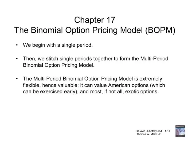
43. Two Step Binomial Trees • We can extend the analysis to two-period binomial trees (and both authors later extend them to multi-period binomial trees). • Here we assume the stock price starts at $20 and that u is 1.1 and d is 0.9 in each of the two time steps. • Suppose that each time step is three months in length and the risk-free rate is 12%. Again consider an option with strike of $21. 24.2 22 19.8 20 18 16.20

44. Two Step Binomial Trees • We want to know the value of the option at time 0. • We begin at the terminal time step of the lattice. Note that at the bottom and middle nodes, the value of the option is 0, while at the top node it is worth 3.2 dollars. 24.2 cuu=max(0,24.2-21)=3.2 22 19.8 cud=max(0,19.80-21)=0 20 18 16.20 cdd=max(0,16.20-21)=0

45. Two Step Binomial Trees • At the second time step we have two nodes to consider. At the bottom node it must be worth zero, since it will be worth zero at time 2 with certainty. • What about at the upper node? To do this we need to calculate some numbers. First, let’s notice a few facts: u = 1.1 d = .9 r = .12 T = .12 • Therefore: p= (e.03 - .9)/ (1.1 - .9) = .6523 (same as before) • and so we can use our standard formula to get the price: e-.12*.25(.6523*3.2 + .3477*0) = 2.0257. • So now we go back to time 0 and do the same thing. P works out the same, so therefore the price is: e-.12*.25(.6523*2.0257 + .3477*0) = 1.2823

46. General Result • This can be seen in the lattice at time 1, 24.2 cuu=max(0,24.2-21)=3.2 22 cu=2.20257 19.8 cud=max(0,19.80-21)=0 20 18 cd=0 16.20 cdd=max(0,16.20-21)=0

47. General Result • As well as at time 0: 24.2 cuu=max(0,24.2-21)=3.2 22 cu=2.20257 19.8 cud=max(0,19.80-21)=0 20 c0=1.2823 18 cd=0 16.20 cdd=max(0,16.20-21)=0

48. Two-Step Binomial Trees • Its neat to see the full lattice, but sometimes its more convenient to work with simply the option values. • We see that after each time step the stock is worth either Su or Sd where S is its initial value. We then calculate the terminal values of fuu and fdd and fud. Then we need to know the values of fu and fd: fu = e-rT[pfuu + (1-p) fud] fd = e-rT[pfud + (1-p) fdd] and ultimately f = e-rT[pfu + (1-p) fd] substituting in gives: f = e-r2T[p2fuu + 2p(1-p)fud + (1-p)2fdd].

49. Cox, Ross, Rubinstein Model • Now ultimately, what determines our model is how we calculate u and d. The most famous model is the one published by Cox, Ross and Rubinstein. In that model they make the following definitions: • Where σ is the volatility of the stocks returns. Using the same value for p as before, then p = (erΔt – d)/(u-d)

50. Cox, Ross, Rubinstein Model • Now notice also that we have the parameter Δt. • This is the amount of time that passes between levels of the lattice. • Some books will refer to this quantity as dt, others as h. • You need to be aware of the fact that there are 3 parameters that held define time in any binomial lattice. • T – the time to maturity (in years) of the option you are pricing. • Δt – the “time step”, or amount of time between levels of the lattice. • N – the total number of levels (i.e. “time steps”) in the lattice. • Realize that Δt=T/N. • Frequently you are given two of these and have to determine the third parameter. · · · · · · N=4 · · · Δt · T