Download
1 / 89
890 likes | 903 Views
Chapter 2: Demand and Supply. 2.1 Demand 2.2 Supply 2.3 Equilibrium 2.4 Elasticity. 2.1 Demand & Supply in Perfect Competition. Assume a large number of buyers and sellers of a good with full information No one buyer or seller has any market power; individuals are “price-takers”

E N D
Chapter 2: Demand and Supply 2.1 Demand 2.2 Supply 2.3 Equilibrium 2.4 Elasticity
2.1 Demand & Supply in Perfect Competition • Assume a large number of buyers and sellers of a good with full information • No one buyer or seller has any market power; individuals are “price-takers” • A supply and demand curve exists for every good in every location at one time • Demand and Supply are simplest in a PC (perfect competition) market
Demand: Definition • A schedule showing amounts that will be purchased at different prices during some specified time period, everything else held constant (ceteris paribus) • This could refer to goods and services (goods market) • This could also refer to labour and capital (factor market)
Demand: Origins • Demand for a good or service comes from two areas: 1) Derived Demand –desired to make something else (ie: iron is desired to make cars) 2) Direct Demand –desired to be used/consumed itself (ie: Pepsi Vanilla is desired to be drank)
The Law of Demand • There is an inverse relationship between the quantity of anything that people will want to purchase and the price they must pay to obtain it: • ceteris paribus (all else held equal) • This causes demand curves to be downward sloping • When prices increase, people buy less • When prices decrease, people buy more
A B C Change in Price = Movement along the Demand D E The Individual’s Demand Schedule 5 4 3 Price of Songs ($) 2 1 20 0 10 30 40 50 Number of Songs per Year
Math Note: We always graph P on vertical axis and Q on horizontal axis, but we write demand as Q as a function of P… If P is written as function of Q, it is called the inverse demand: Normal Form: Qd=100-2P Inverse form: P =50 - Qd/2 • Markets are defined by: • Commodity • Geography • Time.
Change A: Changes in Quantity Demanded A change in a good’s price Causes a change in quantity demanded (the same thing as a movement along the same demand curve)
A Change in Quantity Demanded Originally, song downloadscost $2 5 4 Due to a tax, song downloadsincrease to $3 3 Price of Songs ($) 2 1 D1 D3 30 0 20 40 50 60 70 80 Quantity of Songs Demanded
Change B: Shifts in Demand A change in non-price determinants of demand (income, tastes, etc) Causes ashift in demand* *The whole demand schedule
Decrease in Demand Increase in Demand D2 D3 A Shift in the Demand Curve Suppose universities outlaw the use of MP3 Players Suppose the federal government gives every student an Sony Walkman MP3 player 5 4 3 Price of Songs ($) 2 1 D1 30 0 20 40 50 60 70 80 Quantity of Songs Demanded
Non-Price determinants of Demand • 4) Expectations • Future prices • Income • Product availability • 5) Population (market size) 1) Income, wealth 2) Tastes and preferences 3) The price of related goods Complements Substitutes What movement would these factors cause?
Price of Cigarettes, per pack Price of Cigarettes, per pack $4 $2 $2 D D’ 20 20 10 10 Number of Cigarettes smoked per day Number of Cigarettes smoked per day Shift vrs. Movement A policy to discourage smoking (no smoking in public buildings) shifts the demand curve left A tax raises the price of cigarettes, resulting in a movement along the demand curve D
Price of Kraft Dinner Price of Chicken $2 $2 D D D’ D’ 20 20 10 10 Chicken eaten in a month Kraft Dinner eaten in a month Normal vs. Inferior Goods For normal goods, Demand decreases With income For inferior goods, Demand increases When income decreases 30
2.2 Supply • The amount a producer supplies depends on PROFITS, which depend on COSTS • Costsdepend on • the kinds of inputs (factors of production) used • the amount of each input used • prices of inputs used • technology
Supply: Definition • A schedule that shows how much will be supplied at different prices for a given time period, ceteris paribus. • This could refer to goods and services (goods market) • This could also refer to labour and capital (factor market)
The Law of Supply • The price of a product or service and the quantity supplied are directly related, ceteris paribus • This creates an upward sloping supply curve • The higher the price of a good, the more sellers will make available • The lower the price of a good, the fewer sellers will make available
Change A: Change in Quantity Supplied A change in a good’s price Causes A change in quantity supplied. (This is also called a movement alongthe supply curve.)
F G H I Change in Price Movement along The Supply J The Individual Producer’s Supply Schedule Qnty of Songs Supplied Price / (thousands / Song year) 5 4 3 F $5 550 G 4 400 H 3 350 I 2 250 J 1 200 Price of Song ($) 2 1 0 100 200 300 400 500 600 Quantity of Songs Supplied (thousands of constant-quality units per year)
Change B: Shifts in Supply A change in non-price determinants of supply Causes A shift in supply
S2 S1 S2 b a b d c d A Shift in the Supply Curve When supply decreases the quantity supplied will be less at each price: ie: Singers form a union and successfully negotiate higher wages 5 When supply increases the quantity supplied will be greater at each price: ie: producer finds that she can use some cheaper singers from Newfoundland 4 3 Price of Songs ($) 2 1 40 0 20 60 80 100 120 140 Quantity of Songs Supplied (millions of constant-quality units per year)
Non-Price Determinants of Supply • Cost of inputs • Technology and Productivity • Taxes and Subsidies • Price Expectations (in the input market) • Number of firms in the industry How will these shift supply?
2.3 Market Equilibrium • In the Market, buyers and sellers interact, resulting in a • Single Equilibrium of • One Equilibrium Price • One Equilibrium Quantity
Putting Demand and Supply Together: Finding Market Equilibrium (1) (2) (3) (4) (5) Difference Price per Quantity Supplied Quantity Demanded (2) - (3) Constant-Quality (Songs (Songs (Songs Song per year) per year) per year) Condition $5 100 million 20 million 80 million 480 million 40 million 40 million 3 60 million 60 million 0 2 40 million 80 million -40 million 1 20 million 100 million -80 million Excess quantity supplied (surplus) Excess quantity supplied (surplus) Excess quantity demanded (shortage) Excess quantity demanded (shortage)
Excess quantity supplied at price $5 S Market clearing, or equilibrium, price E A B D Excess quantity demanded at price $1 Market Equilibrium: Definition The condition in a market when quantity supplied equals quantity demanded at a particular price; a point from where there tends to be no movement 5 4 QD= QS 3 Price pef Song ($) 2 1 0 20 40 60 80 100 Quantity of Songs (millions of constant-quality units per year)
The Law of Supply & Demand • The price of any good will adjust until the price is such that the quantity demanded is equal to the quantity supplied • A high price will result in excess supply, pushing price down, and a low price will result in excess demand, pushing price up • the market clears resulting in a single market clearing or equilibrium price.
Example: The Market for Cranberries Qd = 500 – 4p QS = -100 + 2p p = price of cranberries (dollars per barrel) Q = demand or supply in millions of barrels per year
a. The equilibrium price of cranberries is calculated by equating demand to supply: • plug equilibrium price into either demand or supply to get equilibrium quantity:
Example: The Market For Cranberries Price 125 Market Supply: P = 50 + QS/2 • P*=100 50 Market Demand: P = 125 - Qd/4 Q* = 100 Quantity
Factor Market Example: Coffee Shop Jobs Ld = 18 – W LS = -10 + W W = Wage (the PRICE of labour) L = Labour (full time workers, the QUANTITY of labour)
a. The equilibrium wage of workers is calculated by equating demand to supply: • plug equilibrium price into either demand or supply to get equilibrium quantity:
Example: Coffee Shop Jobs Wage (Price of Labour) 125 Market Supply: W = 10 + LS • W*=14 50 Market Demand: W = 18 - Ld Q* = 4 L (Quantity of Labour)
Comparative Statics: Shifts in Demand &/or Supply How do you analyze a change in an exogenous variable? 1.) Decide whether Demand &/or Supply is affected. 2.) Decide in which direction the affected • Demand &/or Supply will move. 3.) Use a Demand and Supply diagram to determine the new equilibrium. 4.) Calculate the new equilibrium (if possible)
Comparative Statics: Gas Prices • Summer 2009: Gas prices at equilibrium are $1.07 per liter • Winter arrives and people drive less (shift in demand) • The new market equilibrium is $0.87 per liter • Cold Weather causes a decrease in gas prices
S E2 E1 $0.87 $1.07 D2 D1 Q2 Q1 Winter Gas Prices
Simultaneous Shifts Example of a double shift. • 2 events • 1. supply • 2. demand • only supply P, Q. • only demand P, Q. • Q is guaranteed
S1 S2 E1 E2 P1 P2 D1 D2 Q1 Q2 Increased Price Example
S1 S2 E1 E2 P1 P2 D1 D2 Q1 Q2 Decreased Price Example
Simultaneous Shifts Example of a double shift. Second possibility: • 2 events • 1. supply • 2. demand • only supply P, Q. • only demand P, Q • Pis guaranteed
S1 S2 E1 E2 P1 P2 D1 D2 Q1 Q2 Increased Quantity Example
S1 S2 E1 E2 P1 P2 D1 D2 Q1 Q2 Decreased Quantity Example
Example: The Market for Cranberries p = price of cranberries (dollars per barrel) Q = demand or supply in millions of barrels per year Assume that a plague reduced cranberry supply by 100 and fear of inflection likewise reduced cranberry demand by 100 so that:
a. The new equilibrium price of cranberries is calculated by equating demand to supply: • plug equilibrium price into either demand or supply to get equilibrium quantity:
Example: The Market For Cranberries New Market Supply: P = 100 + QS/2 Price 125 Old Market Supply: P = 50 + QS/2 • POLD=PNew 50 Old Market Demand: P = 125 - Qd/4 QOLD QNew Quantity New Market Demand: P = 100 - Qd/4
2.4 Elasticity: Percentage Change • Which makes more sense? • GDP increases by 1.4% OR GDP increases by $2.1 Billion • Inflation is 3.2% OR “Prices have gone up between 5 cents and $350,000” • Percentage changes are often easier to grasp than the amount of change • Economists often use elasticities to examine percentage change or responsiveness
Price Elasticity of Demand • Price Elasticity of Demand (ЄQ,p) • The responsiveness of quantity demanded of a commodity to changes in its price • Related to the slope, but concerned with percentage changes
… a large fall in price... S1 An increase in supply brings ... … and a small increase in quantity One Impact of a Change in Supply S0 40.00 30.00 Large price change and small quantity change Price (dollars per pizza) 20.00 10.00 5.00 Da 5 20 25 0 10 13 15 Quantity (pizzas per hour)
An increase in supply brings ... S1 … a small fall in price... 15.00 … and a large increase in quantity Another Impact of a Change in Supply… 40.00 S0 Small price change and large quantity change 30.00 Price (dollars per pizza) 20.00 Db 10.00 5 17 20 25 0 10 15 Quantity (pizzas per hour)
Solution: Price Elasticity of Demand Price Elasticity of Demand Percentage change in quantity demanded ЄQ,P Percentage change in price The ratio of the two percentages is a number without units.
When describing the price elasticity of demand, we often ignore the minus sign for % change in Q. Price Elasticity • Example • Price of oil increases 10% • Quantity demanded decreases 1%