Download
1 / 6
60 likes | 178 Views
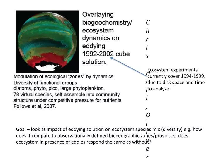
Chris Hill, Oliver Jahn, Stephanie Dutkiewicz Mick Follows. Ecosystem experiments currently cover 1994-1999, due to disk space and time to analyze!.

E N D
Chris Hill, Oliver Jahn, Stephanie Dutkiewicz Mick Follows Ecosystem experiments currently cover 1994-1999, due to disk space and time to analyze! Goal – look at impact of eddying solution on ecosystem species mix (diversity) e.g. how does it compare to observationally defined biogeographic zones/provinces, does ecosystem in presence of eddies respond the same as without?
Conventional, ocean color, view of solution v. SeaWIFS. Top panel – SeaWIFS monthly composite Chl concentration 1998-1999. Bottom panel – cube84 + 78 species self-organizing ecosystem model simulation for 1998-1999. Reasonable, but can now look at what species are contributing to Chl where and when.
Species mix v. space and time – global view. SeaWIFS Chl comparison on previous slide is integral over multiple different species (both in real wolrd and in model). Movie shows concentration of different species categories as a function of space and time. Diatoms (red), prochlorococus (green), picoplankton(blue), everything else(yellow) all contribute to the overall growth rate. At different times at some location different species may dominate. This is driven by relative fitness of the species wrt to local nutrient, light, temperature conditions – but it is also modulated by fluid transport.
Species mix v space and time – local views. Individual species abundance at yellow x as function of time. × The plot and animation show views of abundance of individual species over time at a point. Hofmuller plots of individual species abundance at point on white line.
Connecting to provinces. Model species abundance should be equivalent to “provinces” (Longhurst) – can be compared against observationally inferred provinces. Role of flow can be understood through looking at local growth rate versus actual abundance (which includes fluid transport). Biological “provinces”, M. Oliver et. al (derived from color + SST obs)
Summary • 1994-1999 cube84 + ecosystem new global perspective on species diversity? • may or may not be consistent with province categorization that is being used as a means to monitor ecosystem changes • growth of species assuming local conditions versus actual rate of change can be used to quantify impact of flow/no-flow on species and on nutrients.