Download
1 / 22
250 likes | 533 Views
Introduction to Computer Systems (2). Sequential vs. parallel computing – von Neumann architecture vs. neural networks. Piotr Mielecki Ph. D. http://www.wssk.wroc.pl/~mielecki. mielecki@wssk.wroc.pl. Piotr.Mielecki@pwr.wroc.pl. 1. Sequential vs. parallel data processing.

E N D
Introduction to Computer Systems (2) Sequential vs. parallel computing – von Neumann architecture vs. neural networks. PiotrMielecki Ph. D. http://www.wssk.wroc.pl/~mielecki mielecki@wssk.wroc.pl Piotr.Mielecki@pwr.wroc.pl
1.Sequential vs. parallel data processing. SEQUENTIAL PROCESSING • In mathematics, computing, linguistics, and related disciplines, an algorithm is a finite list of well-defined instructions for accomplishing some task. Algorithm, given an initial state, will proceed through a well-defined series of successive states, possibly eventually terminating in an end-state. • That means we are going trough a sequence of steps from the starting point to the (expected) end. Most of algorithms are composed of a sequence of steps and decisions made according to some conditions. Each decision causes a branch in the sequence –alternative path (see diagram – flowchart).
Lamp doesn’t work (INITIAL STATE) Lamp plugged in? NO Plug in the lamp YES NO NO YES Bulb burned out? NO Doe’s the lamp work? Doe’s the lamp work? YES YES Replace the bulb NO Doe’s the lamp work? Buy new lamp YES Lamp works (END STATE)
SEQUENTIAL PROCESSING • This method of solving the problems is relatively manageable for automation, so most of today’s computers are the sequence automats. That means they are automatically processing data using programmed sequences of operations (with branches in most of cases). • The abstract definition of this kind of automat is the Turing machine, while the “referential model” for real computer was defined by John von Neumann. Key factor of final success is good programming so we need to perform the programming process before using the computer for solving the problem.
PARALLEL PROCESSING • The alternative way of solving the problems, more similar to this used by living biological brain, is not sequential, “logical” rather approach. • To make the decision we are first recognizing the problem reading some impulses/signals from the outside world (information about facts that occurred). Then we are trying to compare the combination of these input impulses with the situation we already know (and we know what to do to succeed). Our decision is based on our knowledge and experience learned before.
INPUT: The problem Impulse #2 Impulse #3 Impulse #1 Impulse #n … KNOWLEDGE AND EXPERIENCE DECISION OUPUT: The solution SOLUTION
PARALLEL PROCESSING • The key factor of well decision-making in this approach is the learning process (instead of programming), performed before. This process has one simple goal: to make finally right decision, that sometimes means “to make possibly smallest mistake (error)”. • One of the elements of learning is simply collecting the information (knowledge), but we can’t assume we have always to deal with already known problems. So. sometimes we have to adapt to quite new situations (just learn new things) • The simplest way of learning may be to compare result reached by the decision with the one assumed as correct – somebody (perhaps a teacher) already knows good solution. In this approach the difference between the “good result” and the result of our last decision (maybe not so good) becomes very valuable information. If we pass this difference (the error signal) back to the input we will have the feedback, which should help us to find (or guess) better decision. This method of learning (passing error signal to input) is called “Error back-propagation method”.
PARALLEL PROCESSING – ERROR BACK-PROPAGATION LEARNING SYSTEM Impulse #1 GOOD RESULT (G) Error (G – R) Impulse #2 Impulse #3 DECISION RESULT (R) … Impulse #n FEEDBACK
PARALLEL PROCESSING • After some iterations, using one or another solution, we should minimize the error signal to zero (or to acceptable low value – the signals here are assumed to be analog, not only 0 or 1), that means we have learned something new (and we should add this knowledge to our knowledge-base). • The data-processing in this model is performed very quickly: just read the input and write the output according to first learned criteria. We could call this “a parallel data-processing” (all the criteria are checked at the same moment), but the term “parallel computing” means something different today (will be discussed later). • Practical implementations of this concept were first done as analog automats, which have feedback adjusted for smoothly driving electric engines and other servomechanisms in industrial machines for example. The structures which are designed exactly for data-processing are based on concept of artificial neuron and the network composed of such neurons (as biological brain is composed of living neurons) called “neural networks”.
ARTIFICIAL NEURON Input x1 Weight #1 w1 x1 Input x2 Weight #2 w2 x2 Weight #3 ∑ S Input x3 t w3 x3 Output (y) … wn xn Threshold function Weight #n 0 S < t Input xn y(S) = 1 S ≥ t
ARTIFICIAL NEURON • In this model input and output signals (xi) of each neuron are assumed to be binary (0 or 1), the weights (wi) associated with inputs have analog values (positive or negative). • The adder (∑) adds all input values multiplied by appropriate weights giving sum (S) on it’s output. • The threshold function y(S) converts output from adder back to binary value (0 if sum is less than assumed t value or 1 if it’s equal or greater than t). • What should we do to build neural network?
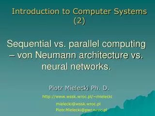
NEURAL NETWORK • Define the connections between set of neurons (topology of the network). • Adjust values of each weight coefficient (wi) for each neuron (notice that if wi = 0 there’s simply no connection between input xi of this neuron with the output of any other neuron nor the input of the entire network). • Adjust the threshold value t of each neuron. • The neural networks used actually in artificial intelligence studies have layered structures, where first-level layer is connected to the input of the entire network (a set of sensors for example) and the last layer is an output. The layers between input and output are virtually hidden, so we can see the entire network as a “black box” with a set of inputs and outputs, we can also implement the feedback between output and input of the network to use error back-propagation based methods in learning process.
LAYERED NEURAL NETWORK Input layer Hidden layers Output layer Input x1 Output y1 Input x2 Output y2 … … Input x3 … Output ym Input xn
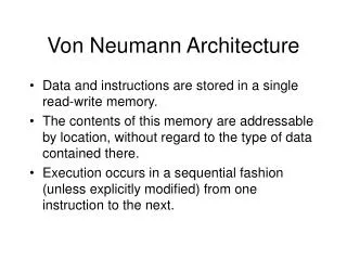
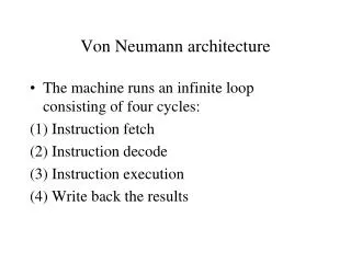
2. Von Neumann architecture as the referential model for sequential computer. DEFINITION The von Neumann architecture is a computer design model that uses a central processing unit (CPU) and a single separate storage structure (memory) to hold both instructions and data. To exchange data with outside world some input/output devices should also be provided. Such a computer implements a universal Turing machine concept, and the common “referential model” of specifying sequential architectures, in contrast with parallel architectures.
The Computer Memory Central Processing Unit (CPU) Arithmetic And Logic Unit (ALU) Control Unit Instruction Pointer Input / Output Outside world
FIXED PROGRAM COMPUTERS The earliest computing machines had fixed programs. Some very simple computers still use this design, either for simplicity or training purposes. For example, a pocket calculator is in most cases a fixed program computer. It can do basic or more sophisticated arithmetic operations, but it cannot be used as a word processor or to run video games. To change the program of such a machine, you have to re-wire, re-structure, or even re-design the machine. Indeed, the earliest (“Generation 0”) computers were not so much “programmed” as they were “designed”. “Reprogramming”, when it was possible at all, was a very manual process, starting with flow charts and paper notes, followed by detailed engineering designs, and then the process of implementing the physical changes (re-wiring in Colossus for example).
STORED PROGRAM COMPUTERS The idea of the stored-program computer changed all that. By creating an instruction set architecture and detailing the computation as a series of instructions (the program), the machine becomes much more flexible. By treating those instructions in the same way as data (storing in the same memory subsystem), a stored-program machine can easily change the program, and can do so under program control (operating system in today’s computers). The terms “von Neumann architecture” and “stored-program computer” are generally used interchangeably. However, the Harvard architecture concept should be mentioned as a design which stores the program in an easily modifiable form, but not using the same storage as for general data.
The CPU in von Neumann machine works according to it’s basic machine cycle, which consists of following steps (elementary operations): Operation code fetch – the CPU reads from memory the word pointed by the register called usually “Instruction Pointer” (IP), then increments this register to address next word in memory. Decoding the operation code – the Control Unit inside CPU chooses which operation should be executed decoding the word read in step a) according to the processor’s instruction set. (Optional) Reading the argument(s) for operation (operands) – if the instruction needs some input data from memory or input/output port, the CPU reads these operands from memory or port either exactly from the word(s) pointed by IP, or from address(es) written in memory next to the operation code. The IP is then incremented by the length of the operand(s) or address(es) if they are read from memory. Executing the instruction – just performing the operation, modifying the operand(s) in most of cases. (Optional) Writing the result of the operation – CPU writes the new value to memory or output port. Go to step a) – the Instruction Pointer now points to the next operation code.
STORED PROGRAM COMPUTERS A stored-program design theoretically lets programs modify themselves while running. One early motivation for such a facility was the need for a program to increment or otherwise modify the address portion of instructions, which had to be done manually in early designs. This became less important when index registers and indirect addressing became customary features of CPU architecture. Self-modifying code is unwanted today since it is hard to understand and debug, and modern processor pipelining and caching schemes make it inefficient.
3.The most well-known problems with stored-program computers. REWRITING THE PROGRAM CODE • In some simple stored-program computers, a malfunctioning program can damage itself by rewriting it’s own code. It can also damage other programs or the operating system, possibly leading to a crash. • A buffer overflow is one very common example of such a malfunction. The ability for programs to create and modify other programs is also frequently exploited by malware. Malware might use a buffer overflow to smash the call stack and overwrite the existing program, and then proceed to modify other program files on the system to propagate the compromise. • Memory protection supported by special hardware and other forms of access control can help protect against both accidental and malicious program modification.
VON NEUMANN’S BOTTLENECK • Other disadvantage of this architecture is phenomena known as von Neumann’s bottleneck. It is caused by the limited throughput (data transfer rate) between the CPU and memory compared to the amount of memory. • In modern machines, throughput is much smaller than the rate at which the CPU can work. This seriously limits the effective processing speed when the CPU is required to perform minimal processing on large amounts of data. The CPU is continuously forced to wait for vital data to be transferred to or from memory. • As CPU speed and memory size have increased much faster than the throughput between them, the bottleneck has become more of a problem. This performance problem is reduced by a cache between CPU and main memory, and by the development of branch prediction algorithms in the CPU microcode.
4. Today’s definition of parallel computing. Parallel computing is the simultaneous execution of some combination of multiple instances of programmed instructions and data on multiple processors in order to obtain results faster. The idea is based on the fact that the process of solving a problem usually can be divided (decomposed) into smaller tasks, which may be carried out simultaneously with some coordination. These small tasks are processed on normal, sequential computers connected with each-other by the fast network or dedicated interfaces or by different processors sharing the same memory in the same machine. There’s large number of different concepts of this kind today.