Download
1 / 45
450 likes | 478 Views
CSE 417: Algorithms and Computational Complexity. Winter 2001 Lecture 9 Instructor: Paul Beame. 1. 2. 10. 3. 11. 12. 4. 8. 13. 5. 9. 6. 7. Undirected Graphs. 1. 2. 10. 3. 11. 12. 4. 8. 13. 5. 9. 6. 7. Directed Graphs.

E N D
CSE 417: Algorithms and Computational Complexity Winter 2001 Lecture 9 Instructor: Paul Beame
1 2 10 3 11 12 4 8 13 5 9 6 7 Undirected Graphs
1 2 10 3 11 12 4 8 13 5 9 6 7 Directed Graphs
Representing Graph G=(V,E)n vertices, medges • Vertex set V={v1,...vn} • Adjacency Matrix A • A[i,j]=1 iff (vi,vj)E • Space is n2 bits • Advantages: • O(1) test for presence or absence of edges. • compact in packed binary form for large m • Disadvantages: inefficient for sparse graphs
4 v1 2 7 3 v2 1 6 v3 5 2 v1 7 vn Representing Graph G=(V,E)n vertices, medges • Adjacency List: • O(n+m) words • O(log n) bits each • Advantages: • Compact for sparse graphs
4 v1 2 7 3 v2 1 6 v3 5 2 v1 7 vn Representing Graph G=(V,E)n vertices, medges • Adjacency List: • O(n+m) words • O(log n) bits each • Back pointers and cross pointers allow easier traversal and deletion of edges • usually assume this format
Graph Traversal • Learn the basic structure of a graph • Walk from a fixed starting vertex v to find all vertices reachable from v • Three states of vertices • undiscovered • discovered • completely-explored
Breadth-First Search • Completely explore the vertices in order of their distance from v • Naturally implemented using a queue
BFS(v) 1 2 3 4 6 7 9 5 11 12 10 8 13
BFS(v) 1 2 3 4 6 7 9 5 11 12 10 8 13
BFS(v) 1 2 3 4 6 7 9 5 11 12 10 8 13
BFS(v) 1 2 3 4 6 7 9 5 11 12 10 8 13
BFS(v) 1 2 3 4 6 7 9 5 11 12 10 8 13
BFS(v) 1 2 3 4 6 7 9 5 11 12 10 8 13
BFS(v) 1 2 3 4 6 7 9 5 11 12 10 8 13
BFS(v) 1 2 3 4 6 7 9 5 11 12 10 8 13
BFS analysis • Each edge is explored once from each end-point (at most) • Each vertex is discovered by following a different edge • Total cost O(m) where m=# of edges
Graph Search Application: Connected Components • Want data structure that allows one to answer questions of the form: • given vertices u and v is there a path from u to v? • Idea : create array A such that A[u] = smallest numbered vertex that is connected to u • question reduces to whether A[u]=A[v]?
Graph Search Application: Connected Components • for v=1 to n doif state(v)!=fully-explored then state(v)discovered BFS(v):setting A[u] vfor each u found endif endfor • Total cost: O(n+m) • each vertex an each edge is touched a constant number of times • works also with DFS
BFS Application: Shortest Paths 0 1 Tree gives shortest paths from start vertex 2 1 3 4 6 7 2 9 5 3 11 12 10 8 can label by distances from start 4 13
Depth-First Search • Follow the first path you find as far as you can go, recording all the vertices you will need to explore further as you go. • Naturally implemented using recursive calls or a stack
DFS(v) 1 2 10 3 11 12 7 8 13 6 9 4 5
DFS(v) 1 2 10 3 11 12 7 8 13 6 9 4 5
DFS(v) 1 2 10 3 11 12 7 8 13 6 9 4 5
DFS(v) 1 2 10 3 11 12 7 8 13 6 9 4 5
DFS(v) 1 2 10 3 11 12 7 8 13 6 9 4 5
DFS(v) 1 2 10 3 11 12 7 8 13 6 9 4 5
DFS(v) 1 2 10 3 11 12 7 8 13 6 9 4 5
DFS(v) 1 2 10 3 11 12 7 8 13 6 9 4 5
DFS(v) 1 2 10 3 11 12 7 8 13 6 9 4 5
DFS(v) 1 2 10 3 11 12 7 8 13 6 9 4 5
DFS(v) 1 2 10 3 11 12 7 8 13 6 9 4 5
DFS(v) 1 2 10 3 11 12 7 8 13 6 9 4 5
DFS(v) 1 2 10 3 11 12 7 8 13 6 9 4 5
DFS(v) 1 2 10 3 11 12 7 8 13 6 9 4 5
DFS(v) 1 2 10 3 11 12 7 8 13 6 9 4 5
DFS(v) 1 2 10 3 11 12 7 8 13 6 9 4 5
DFS(v) 1 2 10 3 11 12 7 8 13 6 9 4 5
DFS(v) 1 2 10 3 11 12 7 8 13 6 9 4 5
1 2 10 3 11 12 7 8 13 6 9 4 5 DFS(v)
Non-tree edges • All non-tree edges join a vertex and its descendent in the DFS tree • No cross edges
Application: Articulation Points • A node in an undirected graph is an articulation point iff removing it disconnects the graph • articulation points represent vulnerabilities in a network
1 2 10 3 11 12 7 8 13 6 9 4 5 Articulation Points
Articulation Points from DFS • Every interior vertex of a tree is an articulation point • Non-tree edges eliminate articulation points • Root nodes are articulation points iff they have more than one child no non-tree edges going from sub-tree below some child of u to above u in the tree non-leaf, non-root node u is an articulation point
DFS Application:Articulation Points root has one child articulation points & reasons 3sub-tree at 4 8sub-tree at 9 10sub-tree at 11 12sub-tree at 13 1 non-tree edges matched with vertices they eliminate 2 3 8 10 4 11 12 9 5 6 leaves are not articulation points 13 7