Download
1 / 57
580 likes | 767 Views
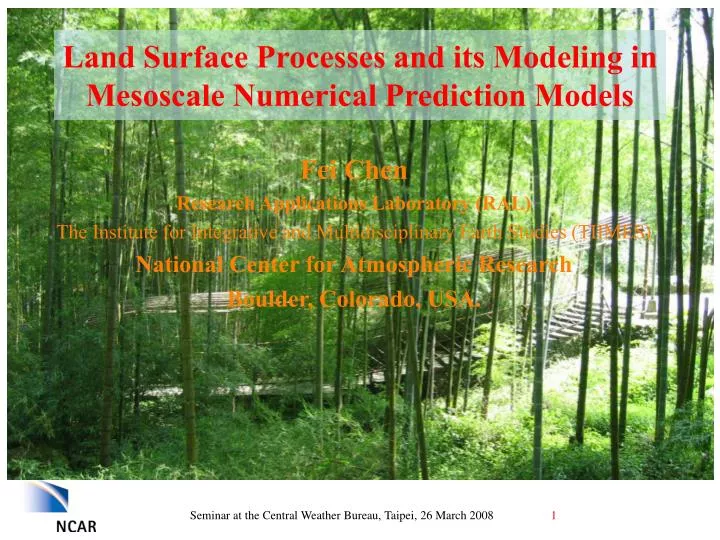
Land Surface Processes and its Modeling in Mesoscale Numerical Prediction Models. Fei Chen Research Applications Laboratory (RAL) The Institute for Integrative and Multidisciplinary Earth Studies (TIIMES) National Center for Atmospheric Research Boulder, Colorado, USA.

E N D
Land Surface Processes and its Modeling in Mesoscale Numerical Prediction Models Fei Chen Research Applications Laboratory (RAL) The Institute for Integrative and Multidisciplinary Earth Studies (TIIMES) National Center for Atmospheric Research Boulder, Colorado, USA. Seminar at the Central Weather Bureau, Taipei, 26 March 2008 1
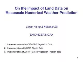
From Dr. Hong Jing-Shan’s overview talk • In NWP aspect, developing the land data assimilation system is critical to improve the forecast in regional-meso scale • Tibetan plateau for springtime system • Mongolian plateau for winter cold surge • Taiwan local circulation (mountain, land-sea breeze, urban interactions) • Improve the local precipitation process • Support the requirement from EPA(Environmental Protection Administration) Seminar at the Central Weather Bureau, Taipei, 26 March 2008 2
Global Precipitation-Soil Moisture Coupling Seminar at the Central Weather Bureau, Taipei, 26 March 2008 3
Effects of Land-use Change on Regional Rainfall Climatology 1993 1900 Evergreen Shrub Crops Marsh June – July Rainfall (mm) 213mm Average rain (238mm) Chen, Pielke, and Mitchell, 2001, chapter in “Observation and Modeling of the Land Surface Hydrological Processes”
Valid 2 June 91 - 29 June 91 0.6 ETA: 80-KM precipitation forecast skills at 36h 0.4 0.2 OSU/Noah LSM Slab model 0.0 2.00 79 1.00 634 0.50 2239 1.50 216 0.10 6637 0.25 4339 0.75 1166 0.01 9660 Rainfall Threshold (In) Impact of Land Surface Model on NWP Quantitative Precipitation Forecast Precipitation Equitable Threat Score OSU/Noah: explicit vegetation, time-varying soil moisture Slab model: simple soil model with fixed soil moisture Chen, Pielke, and Mitchell, 2001, chapter in “Observation and Modeling of the Land Surface Hydrological Processes”
Outline • Overview of land surface processes • Modeling of land surface in mesoscale numerical weather prediction models • Land data assimilation techniques Seminar at the Central Weather Bureau, Taipei, 26 March 2008 6
Earth’s Global Energy Budget • Incident solar flux normalized to “100 units” • Albedo ~ .30: (25 from clouds and 5 from ground) • 70 units still left to be absorbed and re-emitted • 45 units absorbed by the ground, 25 units by the atmosphere • Change of state of water takes a lot of energy: 24 of the 45 units absorbed by the surface used for evaporation Surface affect energy redistribution
Global Water Cycle Surface (ocean and land): source of water vapor to the atmosphere Water Vapour over Land 3 Water Vapour over Sea 10 Net Water Vapour Flux Transport 40 Evapotranspiration 75 Glaciers and Snow 24,064 Precipitation 391 Precipitation 115 Biological Water 1 Evaporation 441 Permafrost 300 Marsh 11 Lake River 2 Soil Moisture 17 Runoff 40 Ground Water 23,400 Sea 1,338,000 State Variable in 1015kg Flux in 1015kg/y Seminar at the Central Weather Bureau, Taipei, 26 March 2008 8
Classic Forms of Boundary Layer Evolution Height Ocean Residual layer Stable boundary layer Potential Temperature Why and how BL over land is different from that over water? Seminar at the Central Weather Bureau, Taipei, 26 March 2008 9
The Atmospheric Boundary Layer (ABL) growth is driven primarily by • Entrainment of warmer air from the free troposphere • Surface sensible and latent fluxes (topic addressing by this lecture). • Also be influenced by the presence of mesoscale phenomena such as the sea-breeze or the mountain valley circulation, due to surface differential heating. Seminar at the Central Weather Bureau, Taipei, 26 March 2008 10
Spatial Variability of PBL on 29 May 02 Contrast between two IHOP-02 western Sites ~50 km apart Site 1 (western Track) Site 3 (western Track) drier, larger sensible heat flux Soil moisture rain Latent heat Net Rad Sensible heat
Outline • Overview of land surface processes • Modeling of land surface in mesoscale numerical weather prediction models • Land data assimilation techniques Seminar at the Central Weather Bureau, Taipei, 26 March 2008 12
Physics Parameterization in NWP Model • Dynamics • Physics • Computers are not yet powerful enough to directly treat them • Processes are not understood well to be represented by an equation • Method of counting for subgrid-scale processes is called parameterization • modeling the effects of a process (emulation) rather than modeling the process itself (simulation). Seminar at the Central Weather Bureau, Taipei, 26 March 2008 13
Why Do We Need Land Surface Models? • Need to account for subgrid-scale fluxes • The lower boundary is the only physical boundary for atmospheric models • LSM becomes increasingly important: • More complex PBL schemes are sensitive to surface fluxes and cloud/cumulus schemes are sensitive to the PBL structures • NWP models increase their grid-spacing (1-km and sub 1-km). Need to capture mesoscale circulations forced by surface variability in albedo, soil moisture/temperature, landuse, and snow • Not a simple task: tremendous land surface variability and complex land surface/hydrology processes • Initialization of soil moisture/temperature is a challenge Seminar at the Central Weather Bureau, Taipei, 26 March 2008 14
An LSM must provide 4 quantities toparent atmospheric model • surface sensible heat flux QH • surface latent heat flux QE • upward longwave radiation QLu • Alternatively: skin temperature and sfc emissivity • upward (reflected) shortwave radiation aQS • Alternatively: surface albedo, including snow effect Seminar at the Central Weather Bureau, Taipei, 26 March 2008 16
Two Important Transport Mechanisms • Molecular conduction of heat, diffusion of tracers, and viscous transfer of momentum cause transport between the surface and the lowest millimeters of air diffusion • Diffusivity for heat, and water vapor: ~ 10-5 m2s-1 • Require large gradient (e.g., 104 Km-1) • Can be neglected above the lowest few centimeter • Turbulent fluxes: • Diffusion coefficient depend on height, wind speed, friction, instability: ~ 100 m2s-1, about 104-105 larger than molecular diffusivity • Caused by small and large eddies: very efficient Seminar at the Central Weather Bureau, Taipei, 26 March 2008 17
Noah LSM in NCEP Eta, MM5 and WRF Models(Pan and Mahrt 1987, Chen et al. 1996, Chen and Dudhia 2001, Ek et al., 2003) Canopy Water Evaporation Transpiration Turbulent Heat Flux to/from Snowpack/Soil/Plant Canopy Precipitation Condensation on vegetation Deposition/ Sublimation to/from snowpack Direct Soil Evaporation Evaporation from Open Water on bare soil Runoff Snowmelt D Z = 10 cm Soil Heat Flux Soil Moisture Flux D Z = 30 cm D Z = 60 cm Internal Soil Heat Flux Internal Soil Moisture Flux Interflow D Z = 100 cm Gravitational Flow
Develop the Advanced Noah Land Surface Modeling System for WRF • Multi-institutional collaborative effort among NCEP, NCAR, U.S. Air Force Weather Agency, NASA, and university community for NWP community • Designed for high-resolution realtime weather forecast, air pollution, local and regional hydrologic applications • Relatively simple, robust, efficient • Noah implemented/tested in • Operational NCEP models: • NAM (12-km, 60-layer) regional model and data assimilation system • GFS global forecast model • GFDL hurricane model • 25-year Regional Reanalysis system (32-km, 60-layer) • AFWA: global land data assimilation system (AGRMET) • NCAR community mesoscale models • MM5 mesoscale model • WRF mesoscale model • Coupled WRF/Noah operational: • AFWA: WRF-ARW for operations July 2006 • NCEP: WRF-NMM for operations June 2006
Noah LSM in WRF V2.2 (Dec 2006) • Improved Physics • Frozen-ground physics • Patchy snow cover, time-varying snow density and snow roughness length • Soil heat flux treatment under snow pack • Modified soil thermal conductivity • Seasonal surface emissivity • Simple treatment of urban landuse • Additional background fields • Monthly global climatology albedo (0.15 degree) • Global maximum snow albedo database • Import various sources of soil data • NCEP Eta/EDAS (40-km): 4-layer soil moisture and temperature • NCEP AVN/GFS/Reanalysis: 2-layer soil data • AFWA AGRMET: global land data assimilation system (47-km) • NCEP NLDAS: North-American land data assimilation system (1/8 degree); 4-layer soil data • NCAR HRLDAS 4-layer soil data • WRF/Noah coupled to a single-layer urban canopy mode Seminar at the Central Weather Bureau, Taipei, 26 March 2008 20
Key References for the Noah LSM • Physics (1-d column model) • Warm season • Chen et al. (1996, JGR, 101) • Cold season (snowpack and frozen soil) • Koren et al. (1999, JGR, 104) • In Mesoscale models • NCEP Eta model • Chen et al. (1997, BLM, 85) • Ek et al. (2003, JGR, 108) • NCAR MM5 model • Chen & Dudhia (2001, MWR, 129) Seminar at the Central Weather Bureau, Taipei, 26 March 2008 21
Key Input to the Noah LSM • Land-use (vegetation) type • Soil texture • Secondary parameters can be specified as function of the above three primary parameters Seminar at the Central Weather Bureau, Taipei, 26 March 2008 22
1-km Global Landuse Map determine Rc_min, and other vegetation parameters Seminar at the Central Weather Bureau, Taipei, 26 March 2008 23
AVHRR vs MODIS land-use data set Seminar at the Central Weather Bureau, Taipei, 26 March 2008 25
Global Soil Texture Map determine Kt, and other soil parameters Seminar at the Central Weather Bureau, Taipei, 26 March 2008 26
Key Input to the Noah LSM • However, some secondary parameters can be specified as spatial 2-D fields (i.e., like gridded primary fields) • The following parameters can be specified either from the table or from 2-d data • Albedo • Green vegetation fraction • Leaf area index • Maximum snow albedo Seminar at the Central Weather Bureau, Taipei, 26 March 2008 28
Seasonality of vegetation Based on monthly NDVI Seminar at the Central Weather Bureau, Taipei, 26 March 2008 29
Seminar at the Central Weather Bureau, Taipei, 26 March 2008 30
Comparison of MODIS 12 June 2002 realtime data and WRF June climatology • MODIS green vegetation fraction lower over most of the domain Seminar at the Central Weather Bureau, Taipei, 26 March 2008 31
Noah LSM Physics in WRF: Overview • Four soil layers (10, 30, 60, 100 cm thick) • Prognostic Land States • Surface skin temperature • Total soil moisture at each layer (volumetric) • total of liquid and frozen (bounded by saturation value depending on soil type) • Liquid soil moisture each layer (volumetric) • can be supercooled • Soil temperature at each layer • Canopy water content • dew/frost, intercepted precipitation • Snowpack water equivalent (SWE) content • Snowpack depth (physical snow depth) • Above prognostic states require initial conditions • Provided by WRF Preprocessing System (WPS) (former SI and REAL) Seminar at the Central Weather Bureau, Taipei, 26 March 2008 32
Noah LSM Physics : Soil Prognostic Equation Soil Moisture • “Richard’s Equation for soil water movement • D, K functions (soil texture, soil moisture) - represents sources (rainfall) and sinks (evaporation) Soil Temperature - C, functions (soil texture, soil moisture) - Soil temperature information used to compute ground heat flux Seminar at the Central Weather Bureau, Taipei, 26 March 2008 33
Noah LSM Physics: Surface Water Budget(Exp: monthly, summer, central U.S.)dS = P - R - E Where: dS = change in soil moisture content - 75 mm P = precipitation 75 R = runoff 25 E = evaporation 125 Evaporation is a function of soil moisture and vegetation type, rooting depth/density, green vegetation cover Seminar at the Central Weather Bureau, Taipei, 26 March 2008 34
Noah LSM Physics: Surface EvaporationE = Edir + Et + Ec + Esnow • E: total surface evaporation from combined soil/vegetation • Edir: direct evaporation from soil • Et: transpiration through plant canopy • Ec: evaporation from canopy-intercepted rainfall • Esnow: sublimation from snowpack Seminar at the Central Weather Bureau, Taipei, 26 March 2008 35
Noah LSM Physics: Vegetation Transpiration (Et) • Et represents evaporation of water from plant canopy via uptake from roots in the soil, which can be parameterized in terms of “resistances” to the “potential” flux Flux = Potential/Resistance • Potential evaporation: amount of evaporation that would occur if a sufficient water source were available. Surface and air temperatures, insolation, and wind all affect this Seminar at the Central Weather Bureau, Taipei, 26 March 2008 36
Noah LSM Physics: Canopy Resistance • Canopy transpiration determined by: • Amount of photosynthetically active (green) vegetation. • Green vegetation fraction (Fg, GVF) partitions direct (bare soil) evaporation from canopy transpiration: Et/Edir ≈ f(Fg) • Not only the amount, but the TYPE of vegetation determines canopy resistance (Rc): Seminar at the Central Weather Bureau, Taipei, 26 March 2008 37
Canopy Resistance (continued) • Where: • LAI: leaf area index • Rc_min ≈ f(vegetation type) • F1 ≈ f(amount of PAR:solar insolation) • F2 ≈ f(air temperature: heat stress) • F3 ≈ f(air humidity: dry air stress) • F4 ≈ f(soil moisture: dry soil stress) • Thus: hot and dry air, dry soil lead to stressed vegetation and reduced transpiration Seminar at the Central Weather Bureau, Taipei, 26 March 2008 38
Canopy Resistance (continued) Jarvis Scheme vs Ball-Berry Scheme Jarvis scheme LAI – Leaf Area Index, F1 ~ f (amount of PAR) F2 ~ f(air temperature: heat stress) F3 ~ f(air humidity: dry air stress) F4 ~ f(soil moisture: dry soil stress) Fundamental difference: evapotranspiration as an ‘inevitable cost’ the foliage incurs during photosynthesis or carbon assimilation An: three potentially limiting factors: 1. efficiency of the photosynthetic enzyme system 2. amount of PAR absorbed by leaf chlorophyll 3. capacity of the C3 and C4 vegetation to utilize the photosynthesis products Ball-Berry scheme in GEM (Gas Exchange Model) hs – relative humidity at leaf surface ps – Surface atmospheric pressure An – net CO2 assimilation or photosynthesis rate Cs – CO2 concentration at leaf surface m and b are linear coeff based on gas exchange consideration
WRF/Noah simulated typical summer surface fluxes and PBL depth Surface fluxes at a wet grassl site Red: latent Green: sensible Surface fluxes at a dry grass site Red: latent Green: sensible Lowest model level RH Red: dry grass Green: wet grass PBL depth Red: dry grass Green: wet grass
WRF/ Noah Snow Storm Case 18 March 2003 24-h snow water equivalent change valid at 00Z 19 March Snow melted too quickly in the OSULSM Obs 24-h SWE change valid at 06Z 19 March Seminar at the Central Weather Bureau, Taipei, 26 March 2008 42
Noah improvement planned for near futureCollaborating with NCEP, NASA, and university groupsFunded by NSF, NOAA, NASA, AFWA, DTRA • Groundwater model • Multi-layer snowpack and new snow cover • Dynamic vegetation • Multi-layer vegetation canopy • Ball-Berry canopy resistance • Snow albedo treatment • Irrigation treatment • 2-D high-res explicit routing • van Genuchten soil hydraulics • Spatially varying soil layer thickness • Unified surface layer (aerodynamic conductance) treatment over land • Multi-layer urban model Seminar at the Central Weather Bureau, Taipei, 26 March 2008 43
Subsurface Flow Routing Noah-Router (NCAR Tech Note: Gochis and Chen, 2003) • New Parameters: Lateral Ksat, n – exponential decay coefficient • Critical initialization value: water table depth • 8-layer soil model (2m – depth) • Quasi steady-state saturated flow model, 2-d (x-,y-configuration) • Exfiltration from fully-saturated soil columns Surface Exfiltration from Saturated Soil Columns Lateral Flow from Saturated Soil Layers Saturated Subsurface Routing Wigmosta et. al, 1994 Seminar at the Central Weather Bureau, Taipei, 26 March 2008 44
WRF/Noah LSM/Urban-Canopy Coupled Model • Single layer urban-canopy model (UCM, Kusaka et al., 2004) • Noah handle natural surfaces, UCM treats man-made surfaces • 2-D urban geometry (orientation, diurnal cycle of solar azimuth), symmetrical street canyons with infinite length • Shadowing from buildings and reflection of radiation • Multi-layer roof, wall and road models Seminar at the Central Weather Bureau, Taipei, 26 March 2008 45
Application of the WRF/Noah/UCM to Taipei27, 9, 3, and 1 km grid spacing, 16 June 2006 case Lin et al. 2008, Atm. Envi. Seminar at the Central Weather Bureau, Taipei, 26 March 2008 46
Application of the WRF/Noah/UCM to Taipei (cont)27, 9, 3, and 1 km grid spacing, 16 June 2006 case Urban heat island PBL evolution Lin et al. 2008, Atm. Envi. Seminar at the Central Weather Bureau, Taipei, 26 March 2008 47
Outline • Overview of land surface processes • Modeling of land surface in mesoscale numerical weather prediction models • Land data assimilation techniques Seminar at the Central Weather Bureau, Taipei, 26 March 2008 48
(a) MM5 initialized with EDAS soil fields (b) MM5 initialized with HRLDAS soil fields Mesoscale models need to capture atmospheric boundary layer structures and motions resulted from surface forcing Simulation with EDAS soil fields put TX convection in wrong area (Trier, Chen, Mannng, 2004, Mon. Wea. Rev.) Seminar at the Central Weather Bureau, Taipei, 26 March 2008 49
Motivation • Mesoscale models need to capture atmospheric boundary layer structures resulted from surface forcing • No routine high-resolution soil observation network • Ultimate approach is to combine observation (including satellite), modeling, and data assimilation • Alternatives: Using observed rainfall, analyzed downward solar radiation, and atmospheric analysis to drive LSMs in uncoupled mode • NCEP NLDAS: North America, 1/8 degree • AFWA ARGMET: global, 47-km, long-term archive • NCAR High-resolution land data assimilation System (HRLDAS). Seminar at the Central Weather Bureau, Taipei, 26 March 2008 50
NCAR High-Resolution Land Data Assimilation System (HRLDAS) Concept Run uncoupled LSM on the same grid as mesoscale NWP models • Using the same LSM as in coupled NWP model: same soil moisture climatology • No Mis-match of terrain, land use type, soil texture, physical parameters between sources of soil data and NWP models • No interpolation and soil moisture conversion Seminar at the Central Weather Bureau, Taipei, 26 March 2008 52
High-resolution Land surface and urban modeling and assimilation system(Chen et al. 2006, JAMC) snow Leaf area index Vegetation type Urban type Vegetation cover Soil texture Terrain Obs. Precipitation Radiation, T, Q, U, V High resolution land data assimilation system (HRLDAS) Soil moisture, soil temperature, snow cover, canopy water, wall/roof/road temperature Noah land surface model, Urban canopy model Boundary layer parameterization Coupled mode
HRLDAS: Capturing Small-Scale Variability • Input: • 4-km hourly NCEP Stage-II rainfall • 1-km landuse type and soil texture maps • 0.5 degree hourly GOES downward solar radiation • 0.15 degree AVHRR vegetation fraction • T,q, u, v, from model based analysis • Output: long term evolution of multi-layer soil moisture and temperature, surface fluxes, and runoff 4-km HRLDAS surface soil moisture in IHOP domain 12 Z May 29 2002 Seminar at the Central Weather Bureau, Taipei, 26 March 2008 54
HRLDAS Surface layer (top 10 cm soil) volumetric soil moisture Initial time From coarse resolution of EDAS field 46 days later Heterogeneity was developed in the 4-km domain Seminar at the Central Weather Bureau, Taipei, 26 March 2008 55