Download
1 / 48
480 likes | 489 Views
Simple Thematic Mapping in Stata. 3 rd German Stata Users Group Meeting Berlin, 8 April 2005. Maurizio Pisati University of Milano Bicocca – Italy maurizio.pisati@unimib.it. Thematic maps.

E N D
Simple Thematic Mappingin Stata 3rd German Stata Users Group Meeting Berlin, 8 April 2005 Maurizio Pisati University of Milano Bicocca – Italy maurizio.pisati@unimib.it
Thematic maps • Thematic maps represent the spatial distribution of one or more variables of interest within a given geographical unit
Thematic maps • Examples: • A sociologist could use a choropleth map (a.k.a. shaded map) to show how the percentage of families below the poverty line varies across the states or the provinces of a given country • A police officer could be interested in analyzing a dot map showing the locations of drug markets within a given city
Software for thematic mapping • Usually, to produce state-of-the-art thematic maps one has to resort to specialized software (e.g., ArcView, MapInfo) • In some cases, however, it is possible to exploit the graphical engine of a general-purpose statistical package to draw simple but effective thematic maps
Stata’s mapping capabilities • Up until version 7, Stata offered very limited mapping capabilities • On the other hand, the graphical engine introduced in Stata 8 is quite flexible and makes it possible to draw several kinds of maps in a relatively simple manner
The tmap package • The tmap package is a suite of Stata programs designed to draw five kinds of thematic map: • Choropleth maps • Proportional symbol maps • Deviation maps • Dot maps • Label maps
The tmap package • Choropleth, proportional symbol, and deviation maps are intended to depict area data • Dot maps are suitable for representing point data • Label maps can be used to show data of both types
The tmap package • The tmap package exploits the possibility – offered by the new Stata graphical engine – to overlay a large number of different graphs, each of which is used to create a distinct element of the desired map
The tmap package • Specifically: • graph twoway area is used to draw the outlines of the geographical areas of interest and to fill them with the appropriate colors • graph twoway scatter is used to plot the proper symbols or labels when required
Required datasets • To use tmap, one typically needs two Stata datasets: • The master dataset • The boundary dataset
Master dataset • The master dataset is intended to store the spatial data to be represented • It is a standard cases-by-variables dataset whose rows represent the geographical areas or locations objects of analysis
Master dataset: example id land turnout 1 Baden-Wuerttemberg 62.6 2 Bayern 57.1 3 Bremen 61.3 4 Hamburg 68.7 5 Hessen 64.6 6 Niedersachsen 67.0 7 Nordrhein-Westfalen 56.7 8 Rheinland-Pfalz 62.1 9 Saarland 55.5 10 Schleswig-Holstein 66.5 11 Brandenburg 56.4 12 Mecklenburg-Vorpommern 70.6 13 Sachsen 59.6 14 Sachsen-Anhalt 56.5 15 Thueringen 53.8 16 Berlin 68.1
Boundary dataset • The boundary dataset is intended to store the geographical boundaries of the whole geographical unit of interest R or of its sub-areas Ai (i = 1,…,n)
Boundary dataset • The boundary dataset must always include the following three variables: • _ID, which contains the numeric identifier of R or of each sub-area Ai • _X, which contains the x-coordinates of the polygon or polygons that make up R or each sub-area Ai • _Y, which contains the y-coordinates of the polygon or polygons that make up R or each sub-area Ai
Boundary dataset • If one or more of the sub-areas Ai are “islands”, i.e., are completely surrounded by the territory of another sub-area, then the boundary dataset must include an additional variable: • _ISLAND, which takes value 1 when the corresponding sub-area is an “island”, and value 0 otherwise
Boundary dataset • The boundary dataset must always be sorted by variable _ID
Boundary dataset • Each polygon included in the boundary dataset must be defined by 1+k+1 records, each of which corresponds to a proper pair of (x,y) coordinates
Boundary dataset • The first record denotes the beginning of a new polygon and corresponds to a missing coordinate pair (.,.)
Boundary dataset • The 2nd to (k+1)th records denote the k nodes of the polygon and correspond to the k coordinate pairs (x,y) that define such nodes • These records must be arranged so as to correspond to consecutive nodes
Boundary dataset • The last record denotes the end of the polygon and corresponds to a coordinate pair which is an exact replica of the first node of the polygon
Boundary dataset: example +-------------------------+ | _ID _X _Y _ISLAND | |-------------------------| | 1 . . 0 | <- Polygon 1: start | 1 10 10 0 | | 1 10 30 0 | | 1 18 30 0 | | 1 18 10 0 | | 1 10 10 0 | <- Polygon 1: end | 1 . . 0 | <- Polygon 2: start | 1 22 10 0 | | 1 22 30 0 | | 1 30 30 0 | | 1 30 10 0 | | 1 22 10 0 | <- Polygon 2: end |-------------------------| | 2 . . 0 | <- Polygon 3: start | 2 10 30 0 | | 2 10 50 0 | | 2 30 50 0 | | 2 30 30 0 | | 2 10 30 0 | <- Polygon 3: end |-------------------------| | 3 . . 1 | <- Polygon 4: start | 3 22 48 1 | | 3 28 48 1 | | 3 28 42 1 | | 3 22 42 1 | | 3 22 48 1 | <- Polygon 4: start +-------------------------+
Boundary dataset: mif2dta • mif2dta is a simple Stata program that converts MapInfo Interchange Format boundary files into Stata boundary datasets • mif2dta converts any given pair of files rootname.mif and rootname.mid into a new pair of Stata datasets: rootname-Coordinates.dta (the boundary dataset) and rootname-Database.dta (the master dataset) • Optionally, mif2dta also computes the coordinates of the centroids of the geographical areas of interest
Boundary dataset: shapefiles • To convert a shapefile into a Stata boundary dataset: • Convert the shapefile of interest into the proper pair of MIF files (e.g., using the freeware DOS program shp2mif.exe) • Use mif2dta to convert the MIF files into the corresponding Stata master and boundary datasets
tmap choropleth • tmap choropleth represents the spatial distribution of area data by means of choropleth maps, i.e., maps where each of n sub-areas is colored (or shaded) according to a discrete scale based on the value taken on by a quantitative variable of interest in that sub-area
tmap choropleth • The number of classes that make up the discrete scale must be between 2 and 9 • The corresponding class breaks can be based on four different criteria: • Quantiles • Equal intervals • Standard deviates • Custom
tmap choropleth: example tmap choropleth spd2, /// id(id) map(Germany-Coordinates.dta) /// clmethod(quantile) clnumber(4) /// palette(Reds) /// title("Pct. votes for SPD at latest election") /// subtitle("(Two-party share)") /// legpos(5)
tmap propsymbol • tmap propsymbol represents the spatial distribution of area data by means of proportional symbol maps, i.e., maps where the value taken on by a quantitative variable of interest in each of n sub-areas is represented by a symbol whose size is proportional to the value itself
tmap propsymbol: example tmap propsymbol spd2, /// x(x_coord) y(y_coord) /// map(Germany-Coordinates.dta) /// scolor(red) sshape(O) ssize(1.2) /// ocolor(white) fcolor(sand) /// title("Pct. votes for SPD at latest election") /// subtitle("(Two-party share)") /// note("Symbol size proportional to variable value", span)
tmap deviation • tmap deviation represents the spatial distribution of area data by means of deviation maps, a particular kind of proportional symbol maps where: • symbol size expresses the absolute deviation of the quantitative variable of interest from its mean or median • symbol fill expresses the sign of the deviation (positive or negative)
tmap deviation: example tmap deviation spd2, /// x(x_coord) y(y_coord) /// map(Germany-Coordinates.dta) /// scolor(blue) sshape(O) ssize(1.2) /// ocolor(white) fcolor(bluishgray) /// title("Pct. votes for SPD at latest election") /// subtitle("(Two-party share)") /// note(`"`"Solid circles denote positive deviations from the mean"'"' /// `"`"Hollow circles denote negative deviations from the mean"'"' /// `"`"Circle size proportional to absolute value of deviation"'"', /// span)
tmap label • tmap label is an auxiliary program that allows the user to superimpose onto a base map the values taken on by a numeric or string variable at different locations • This program can be used, for example, to plot sub-area names or to represent the spatial distribution of a given quantitative variable of interest in numeric form
tmap label: example tmap label state, /// x(x_coord) y(y_coord) /// map(Germany-Coordinates.dta) /// lcolor(red) llength(30) lsize(0.8) /// ocolor(sienna) fcolor(eggshell) /// title("Länder")
tmap dot • tmap dot represents the spatial distribution of point data by means of dot maps, i.e., maps where the locations at which some “events” of interest have occurred are indicated by symbols whose color and/or shape can vary according to the type of “event”
tmap dot: example tmap dot, /// x(x) y(y) /// map("MilanoOutline-Coordinates.dta") /// by(type) /// fcolor(stone) /// title("Location of police stations") /// subtitle(`"`"Milano, 2004"'"') /// legtitle("Police force", size(*0.7)) /// legbox(lc(black))
tmap choropleth: more examples tmap choropleth murder if conterminous, /// id(id) map(Us48-Coordinates.dta) /// palette(Blues) ocolor(white) bcolor(navy) /// title(`"`"Murders per 100,000 population & Pct. pop. with high school diploma"'"', /// color(white) span) subtitle("United States 1994", color(white)) /// legbox(lc(white) fc(navy) margin(medsmall)) /// legpos(5) legcol(white) /// legtitle("Murder rate", color(white) size(*0.8)) /// addplot(deviation hsdip if conterminous, x(x) y(y) sc(red) ssi(0.8)) /// note(`"`"Circles represent pct. pop. with high school diploma"'"' /// `"`"Solid circles denote positive deviations from the mean"'"' /// `"`"Hollow circles denote negative deviations from the mean"'"' /// `"`"Circle size proportional to absolute value of deviation"'"', /// color(white) span)
tmap choropleth: more examples tmap choropleth winner if conterminous, /// id(id) map(Us48-Coordinates.dta) /// clmethod(unique) /// palette(Custom) colors(`"`"203 24 29"'"' navy) /// title(US Presidential Elections 2004) /// subtitle(Pct. votes for Bush) /// legpos(5) legsize(1.2) /// legtitle("Winner", size(*0.8)) legcount /// addplot(label votebushpct if conterminous, /// x(x) y(y) lc(gs14) ls(0.9))
tmap and spatial data analysis • tmap can be used to display results produced by other Stata programs, e.g., spatial data analysis programs • What follows is an example of a choropleth map + LISA cluster map (Anselin 1995) created using a combination of tmap and a modified version of spatlsa
European Parliament Elections 2004 - Lombardia Pct. votes for Northern League
Ackowledgments • The color schemes used in tmap choropleth were designed by Dr. Cynthia A. Brewer, Department of Geography, The Pennsylvania State University, University Park, Pennsylvania, USA. The color schemes are used with Dr. Brewer’s permission and are from the ColorBrewer map design tool available at ColorBrewer.org
Ackowledgments • I wish to thank Nick Cox and Ian S. Evans for helping improve the first release of tmap • The second release owes much to ideas and suggestions by Nick Cox and Vince Wiggins • Any remaining errors and limitations are mine