Download
1 / 65
650 likes | 657 Views
Binary Decision Diagrams. Lecture 8 - 28.5.2002 Lecture 9 – 4.6.2002 Lecturer: Karen Yorav. Based on the papers:. “Breadth-First with Depth-First BDD Construction: A Hybrid Approach” Yirng-An Chen, Bwolen Yang, and Randal E. Bryant

E N D
Binary Decision Diagrams Lecture 8 - 28.5.2002 Lecture 9 – 4.6.2002 Lecturer: Karen Yorav
Based on the papers: • “Breadth-First with Depth-First BDD Construction: A Hybrid Approach”Yirng-An Chen, Bwolen Yang, and Randal E. Bryant • “Parallel Breaddth-First BDD Construction”Bwolen Yang and David R. O’Hallaron • Presentation by Assaf Schuster
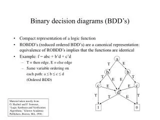
a b c f 0 0 0 0 0 0 1 0 0 1 0 0 0 1 1 1 1 0 0 1 1 0 1 0 1 1 0 0 1 1 1 1 a a b b b b c c c c c c 0 0 0 1 1 0 0 1 0 1 Reduced Ordered BDDs f = (b^c)v(a^!b^!c)
BDD operations • Construction • Boolean Operations • The “apply” function • Restriction • fx=0 = f with x restricted to 0 • fx=1 = f with x restricted to 1 • Variable reordering • not in the scope of this course
r r x op op g op f gx=0 gx=1 fx=0 fx=1 Shannon Expansion r = f op g = !xΛ(fx=0 op gx=0) V xΛ(fx=1 op gx=1)
r x h h Reduction !xΛh V xΛh h r h
Reduction (cont.) • Terminals: • h h = h • h 0 = 0 • h h = h • h 1 = 1 • 0 • 1
Depth First BDD Construction • Apply Shannon expantion on the way down, in a depth first manner • Apply reductions on the way up • Use “unique table” to maintain uniqueness • every sub-BDD is kept in the table • Use “computed cache” to save on computation • Each entry is a tuple (op, f, g, res)
Operator nodes are not created - they exist implicitly in the arguments to recursive calls • top_variable(f, g) • the highest order variable of the two top variables in f and g • (op, f, g) is a terminal case when the result can be computed without further expansion
df_op(op, f, g) : if (terminal case) then return (simplified result); if ((op, f, g) is in computed cache) then return result from cache; x := top_variable(f, g); e := df_op(op, fx=0, gx=0); t := df_op(op, fx=1, gx=1); if (t == e) then return t; result := find or add (x, t, e) in the unique table; insert (op, f, g, result) into the computed cache; return (result);
v1 v1 DF computation op f g
v1 op op v2 v2 v2 v2 DF computation gv1=0 gv1=1 fv1=0 fv1=1
v3 v3 v1 v2 v2 v2 DF computation op op op
v1 v2 v3 v2 v2 DF computation op op op op
v4 v1 v2 v3 v2 v2 DF computation op op op
v4 v4 v1 v2 v3 v2 v2 DF computation op op
v1 v2 v3 v2 v2 DF computation op op And so on ...
Advantages and Disadvantages • No memory overhead • size of memory needed during computation is bounded by the size of the resulting BDD • Poor memory localization • slow operations due to many cache misses and swapping
Breadth First BDD Construction • Apply Shannon expantion in a breadth-first manner. • Reductions are performed on the way up, after all operations are expanded • Operations are stored in “operation nodes”
Data Structure • During the computation the BDD includes 3 types of nodes: • BDD nodes: variable, 0branch, 1branch • Operation nodes: operation, 0branch, 1branch • Forwarding nodes: result • A node can be transformed from one type to another by changing values of fields (the type field).
op f g v1 v1 BF computation
op op op v2 v2 v2 v2 gv1=0 gv1=1 fv1=0 fv1=1 BF computation
op v3 v3 op op op op v2 v2 BF computation
op op v3 v3 v3 v3 op op op op op BF computation
op op v3 v3 op op op op v3 BF computation
v3 v3 op op op v3 v3 BF computation
op v2 v2 BF computation
v1 BF computation
f g OR x1 x1 x2 x2 x2 x2 x3 x3 0 1 0 Example: g f
x1 OR x1 x1 x2 x2 x2 x2 x3 x3 0 1 0 f g Example: g f OR
x2 x2 x1 x1 x1 x2 x2 x2 x2 x3 x3 0 1 0 f g Example: g f OR
x3 x2 x2 x1 x1 x1 x2 x2 x2 x2 x3 x3 0 1 0 f g Example: g f
x2 x2 x1 x1 x1 x2 x2 x2 x2 x3 x3 0 1 0 f g Example: g f F
x2 x2 x1 x1 x1 x2 x2 x2 x2 x3 x3 0 1 0 f g Example: g f
x2 x1 x1 x1 x2 x2 x2 x2 x3 x3 0 1 0 f g Example: g f
Data Structure (cont.) • For each variable vi there is an operation queueopQi • opQi holds operation nodes for which the top_variables of the operands is vi • For each variable vi there is a reduce queueredQi • redQi holds unreduced operation nodes for vi that were created during expantion • During the reduction phase these will be turned into BDD nodes
Data Structures (cont.) • The Unique Table • A hash table of all BDD nodes • The Compute Cache • caching of operation results to prevent recomputation
bf_op(op, f, g) opNode := preprocess_op(op, f, g); if (opNode is a BDD node) then { return opNode; } else { expand(); reduce(); }; return opNode.result;
preprocess_op(op, f, g): if terminal case then return simplified result; if (op, f, g) is in compute_cache then { return result from compute_cache } else { opNode := (op, f, g); i := top_variable(f, g); add opNode to opQi; insert opNode into compute_cache; return opNode; }
expand() : foreach opQi starting from the top most i foreach opNode in opQi: (op, f, g) := opNode opNode.branch0 := preprocess_op(op, fx=0, gx=0) opNode.branch0 := preprocess_op(op, fx=0, gx=0) add opNode to redQi
reduce() : foreach variable vi starting from the bottom variable foreach opNode in redQi (op, f, g) := opNode; if opNode.branch0 is a BDD res0 := opNode.branch0 else res0 := opNode.branch0.result; if opNode.branch0 is a BDD res0 := opNode.branch0 else res0 := opNode.branch0.result;
if (rew0 == res1) then opNode.result = res0 else { b := BDD node (x, res0, res1) opNode.result := lookup(unique_table, b); if BDD node b not in the unique table then { insert b into the unique table opNode.result := b; }; };
Advantages and Disadvantages • Memory localization • special memory manager • separate compute_cache and unique_table for each vi • Considerable memory overhead
Hybrid Approach • Expand in Breadth-first manner until threshold reached • Continue in Depth-first manner • Control memory overhead • Utelize memory localization as much as possible
Partial Breadth-First Algorithm • Start expantion as Breadth-first • Whenever a threshold is reached - • partition remaining operations in groups • handle each group in the regular breadth-first manner • finish reducing one group before expanding the next
Contexts • A Context includes all the information of the algorithm when stopped in the middle: • a range of variables handled: min_i - max_i • a partitioning of all remaining operations into groups • Snapshot of reduce queues • The unique_table and compute_cache are not part of the context • they continue to accumulate throughout the algorithm
Context Stack • New context • Starts with a given list of groups of operations • All opQ’s and redQ’s are empty • Pushing a context • puts the context information on the stack (operation groups + redQ’s) • Empties all opQ’s and redQ’s • Popping a context • restores list of operation groups • restores all redQ’s
top_context • The current context being processed. Includes: • a list of groups of operations ( (list_of_op_nodes1, list_of_op_nodes2 ...) • redQi for each vi • When a context is saved, only the list of groups is saved, the operations in the opQ’s continue as the new context
pbf_op(op, f, g) opNode := preprocess_op(op, f, g); if (opNode is a BDD node) then { return opNode; } else { top_context :=initial context; -- top operation while (context_stack or top_context) { if top_context= empty then top_context := pop(context_stack); remove next group of operations from top_context insert each operation to the proper opQi lexp: expand(); reduce(); }; }; return opNode.result;
expand() : nOpsProcessed := 0 foreach opQi starting from the top most i foreach opNode in opQi: (op, f, g) := opNode opNode.branch0 := preprocess_op(op, fx=0, gx=0) opNode.branch0 := preprocess_op(op, fx=0, gx=0) add opNode to redQi nOpsProcessed++; if (nOpsProcessed > evalThreshold) then { push top_context onto context stack partition remaing operations into groups create a new context from these groups update top_context to the new context goto lexp; -- start the new context }