Download
1 / 32
320 likes | 525 Views
Introduction to Binary Decision Diagrams. - Shesha Shayee K. Raghunathan. Objective. This presentation is about introducing a data structure known as Binary Decision Diagram (BDD for short) and the manipulations that can be performed on them.

E N D
Introduction to Binary Decision Diagrams - Shesha Shayee K. Raghunathan University of Southern California
Objective • This presentation is about introducing a data structure known as Binary Decision Diagram (BDD for short) and the manipulations that can be performed on them. • It is also hoped that this presentation gives an insight in understanding as to why BDDs are so prevalent and its relevance in modern day Logic and Sequential Design. University of Southern California
Agenda • Definitions and Notations • Representations of Boolean Functions- Classical • Representation of Boolean Functions – BDD • BDD – Definitions • The ITE operator • BDD – Advantages and Issues • BDD - Operations • Implementation Techniques • Summary References University of Southern California
Overview • Topic: BDD is a data structure that represents the Logical or Boolean functions in an efficient and in an effective manner for most conditions as compared to other representations. • Presentation: Presentation begins by providing some basic background about Boolean Algebraic functions and its representation. It then proceeds to describing the way it can be represented using BDDs. BDDs are then introduced more formally and the conditions, constraints and properties of this data structure are presented. Then the operations and manipulations that can be performed on BDDs are introduced. Advantages of BDDs are then enumerated. Summary of this presentation then follows after which some references are provided. University of Southern California
Vocabulary • BDD- Binary Decision Diagram ( Unless otherwise specified BDD in this presentation represents an Ordered BDD ) • ROBDD - Reduced Ordered Binary Decision Diagram • ITE – If Then Else operator University of Southern California
1. Definitions and Notations • Boolean Variables : These are variables that can take either 0 or 1 (also known as Boolean Space) as its values. x <- { 0 , 1 } Here {0,1} represents Boolean Space and ‘x’ the Boolean Variable. • Boolean Function : This is a mapping of one or more variables from a Boolean Space of the order of the number of variables to a Boolean Space of single order. f : B^n --> B Here ‘f’ represents a Boolean function, ‘B’ represents the Boolean Space while ‘n’ is the number of boolean variables on which the function is defined. University of Southern California
2. Representation of Boolean Functions -Classical • Disjunctive Normal Form also known as Sum Of Products( SOP ) representation. ex : ab + cd • Conjunctive Normal Form also known as Product Of Sums( POS ) representation. ex : (a+b) (c+d) Here ‘a’ , ‘b’, ‘c’ and ‘d’ are Boolean Variables. University of Southern California
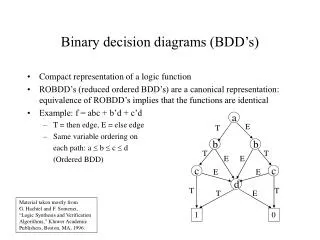
3. Representation of Boolean Functions- BDD Ex : ab + cd a 1 a 0 0 1 b 0 b 1 c 1 c 1 0 0 0 d 1 d 0 0 0 1 0 1 University of Southern California
3.1 BDD Formation – Steps for f = ab + cd 1 1 FINAL STEP 2 STEP 1 STEP 3 a VARIABLE ORDER < < < b c d a a a a 1 1 1 1 0 0 0 0 b b b b 0 0 0 c c c c 1 1 1 1 1 d d 0 0 0 1 0 1 0 University of Southern California
4. BDD - Definitions Def 1 : A function graph is a rooted, directed graph with vertex set V containing 2 types vertices viz non-terminal and terminal. Def 2 : A function graph G having root vertex v denotes a function fv defined recursively as : 1. If v is a terminal terminal vertex: a. If value(v) = 1, then fv = 1 b. If value(v) = 0, then fv = 0 2. If v is a non-terminal vertex with index(v) = i, then fv ( x1, x2, .., xn ) = ~xi . flow(v) ( x1, .. , xn ) + xi . fhigh(v) ( x1, .. , xn) University of Southern California
4.1 BDD – Definitions Contd.. Def 3: Function graphs G and G’ are isomorphic if there exists an one-to-one function g(v)=v’, then either both v and v’ are terminal vertices with value(v) = value(v’) , or both v and v’ are non-terminal vertices with index(v) = index(v’), g( low(v) ) = low(v’), and g( high(v) ) = high(v’) Def 4: A function graph G is reduced if it contains no vertex v with low(v) = high(v), nor does it contain distinct vertices v and v’ such that the sub-graphs rooted by v and v’ are isomorphic. University of Southern California
4.2 BDD – Definitions Contd.. Theorem : For any Boolean function f, there is a unique( up to isomorphism) reduced function graph denoting f and any other function graph denoting f contains more vertices. Def 5 : Restriction or Co-factoring is an operation of changing the graph into a graph for which an input variable is fixed to 0 or 1. University of Southern California
5. TheITEoperator • This is based on the Shannon’s expansion theorem and this is called the ‘If-Then-Else’operator. This is a ternary operator defined as follows: ITE( F, G, H ) = F.G + ~F.H where F, G , H are 3 arbitrary switching functions. • A very important property of theITE operator which is of great interest for this presentation, and for BDD in general, is thatall two-argument operators can be expressed in terms of theITEoperator . • The above mentioned property gives great power to manipulate switching functions and hence are used extensively in manipulating the BDD. University of Southern California
5.1 The ITEoperator - Example ITE( F, G, H) = F.G + ~F.H For sake of simplicity, assume F = x and G = y as the input functions on which manipulations are to be done. Consider ITE( F,G,0 ): ITE( F, G, 0 ) = F.G + ~F.0 = x.y + 0 = x.y Consider ITE( F, 1, G) : ITE( F, 1, G ) = F.1 + ~F.G = x + ~x . y = x + y • The above 2 examples show the powerfulness of, and the simplicity with which ITE operator can be used to express 2 argument operators. University of Southern California
5.2 The ITEoperatortable University of Southern California
5.3 ITEoperator – The Recursive Synthesis Approach We have, ITE( F, G, H ) = F. G + ~F . H By applying Shannon’s Expansion to the above formula gives: ITE( F, G, H ) = x. ( F . G + ~F . H )x +~x . ( F . G + ~F . H )~x where ‘x’ is some Boolean variable, of the 3 functions, on which this expansion is done. ITE( F, G, H ) = x ( Fx . Gx + ~Fx . Hx ) + ~x. ( F~x . G ~x + ~F~x . H~x ) = x ( ITE( Fx , Gx , Hx ) ) + ~x ( ITE( F~x , G~x , H~x ) ) ITE( F, G, H ) = ( x, ITE( Fx , Gx , Hx ) , ITE( F~x , G~x , H~x ) ) Terminal cases for this Recursion are : ITE( 1, F, G ) = ITE( 0, G, F ) = ITE( F,1, 0 ) = ITE( G, F, F ) = F University of Southern California
BDD – Advantages and IssuesAdvantages • The size of the BDD( number of nodes) is exponential in the number of variables in the worst case. • The logical AND and OR of BDD’s have the same complexity . Complementation is inexpensive. • Both satisfiability and tautology can be solved in constant time. • Covering problems can be solved in time linear in the size of the BDD representing the constraints. Note: All the above stated advantages are for BDDs that are Reduced. For more info refer [4] Chapter - 6. University of Southern California
6.1 BDD – Advantages and IssuesIssues • BDD sizes are depend on the ordering of the variables and finding good ordering is not simple. • There are functions for which the SOP or POS representations are more compact than the BDDs. Unfortunately, many constraint functions of covering problems fall into this category. • In some cases, SOP/POS forms are closer to the final implementation of a circuit. Ex : PLA. University of Southern California
6.2 BDD Advantages and IssuesIssues -Variable Ordering Problem Assume Ordering : X1< X2 < X3 < X4 < X5 < X6 X1.X2 + X3. X4 + X5.X6 X1.X3 + X2. X5 + X3.X6 1 1 2 2 2 6 Nodes 14 3 3 3 3 3 4 4 4 4 4 12 Edges 28 5 5 5 6 6 0 1 0 1 University of Southern California
BDD – Operations7.1 Reduction a a 0 1 0 1 b b b b 0 1 1 0 1 0 1 0 c c c 0 0 1 0 1 1 0 1 1 0 0 1 Fig(I) Fig(II) In fig(I) we see that the sub-graphs represented by the ‘c’ node are isomorphic. Hence, the representation contains redundancy. Fig(II) shows the BDD that is obtained after eliminating one of the isomorphic nodes. University of Southern California
7.1 Reduction Contd.. a a 0 1 0 1 b b b 0 1 1 1 0 0 c c 0 1 1 0 0 1 0 1 Fig(III) Fig(II) Fig(II) though removed one of the conditions that caused redundancy in the BDD, it didn’t remove the other possible kind of redundancy as shown in Fig(II) which is present in node ‘ b’. BDD is further reduced to obtain a ROBDD shown in Fig(III). University of Southern California
7.2 The APPLY Operation This is the most important of all the operations that can be performed on the BDDs. • The APPLY operation provides the basic method for creating the representation of a function according to the operators in a Boolean expression or logic gate network. • APPLYtakes graphs representing functions f1 and f2 , a binary operator <op> and produces a reduced graph representing the function f1 <op> f2 defined as : [f1 <op> f2 ] ( x1, x2, … , xn ) = f1(x1, x2, … , xn ) <op> f2 (x1, x2, … , xn ) • The algorithm proceeds from the roots of the 2 argument graphs downward, creating vertices in the result graph at the branching points of the 2 argument graphs. • The control structure of the algorithm is based on the Shannon’s expansion equation/theorem given below: f1 <op> f2 = ~xi . ( f1|xi= 0 <op> f2 |xi = 0 ) + xi . ( f1|xi= 1 <op> f2 |xi = 1 ) University of Southern California
7.2 APPLY* using ITEoperatorAn Example The example presented below is the one that is presented in Bryant’s classic paper. ITE operators are used as they give a straight forward implementation of the APPLY operation. Ex: We want to find ~( a.c ) + b.d using APPLY. Given F = ~(a.c) and G = b .c in the form of a BDD. ~( a . c ) + b . c a b c c 0 1 1 0 University of Southern California
7.2 APPLY Example Contd.. Assume ordering is a < b < c. ITE( ~(a.c) , 1, bc ) a 0 1 ITE( 1, 1 , bc ) = ( 1.1 + 0.bc ) ITE( ~c , 1, bc ) 1 b 0 ITE( ~c, 1, c ) 1 ITE( ~c, 1, 0 ) c 0 1 0 1 ITE( 1, 1, 0 ) = ( 1.1. + 0.0 ) ITE( 0, 1, 0 ) = ( 0.1 + 1.0 ) ITE( 1, 1, 0 ) = ( 1.1 + 0.0 ) ITE( 0, 1, 1 ) = ( 0.1 + 1.1 ) 1 0 1 1 University of Southern California
*Note from Instructor Although this example is called the “Apply operation”, it is halfway between what we call the “Joint ROBBD” and “the Apply Algorithm”. If “ITE” were eliminated from each node in this example, we would have obtained the joint ROBDD for the triple ( ~(a.c) , 1, bc ). After that, we compute the ITE on each of its leaves and reduce to obtain the ROBDD for ITE ( ~(a.c) , 1, bc ). The advantage of this approach is that, for no extra work, the joint ROBDD is now available for any three variable operation, not just the ITE operation, and for almost no extra work. However, there is a disadvantage to doing all this work if only one (in this case, the ITE) operation is desired. In an example as small as this, this disadvantage is not obvious, but suppose the functions (f, g, h) in the ITE operation, ITE(f, g, h), were large and complicated, but that we had already computed each of them and stored them as ROBDDs. Without their unique table, all our work in generating their ROBDDs in the first place would have to be repeated in the process of creating the ROBDD for ITE ( ~(a.c) , 1, bc ). The real power of the Apply Algorithm is that all of this extra work is saved by making use of the functions’ unique tables. If we assume that these unique tables were created and saved as their ROBDDs are obtained, then each cofactor calculation required by the method suggested here is, is replaced with a look-up in the unique table. All of this is not inconsistent with the intentions of the person who created this slide presentation – indeed, he may have intended using the unique table as part of the process he described. Moreover, if unique tables are available, the joint ROBDD process is also enhanced. My point is that, without the unique table, the process described is so inefficient that we might as well compute the joint ROBDD and hope that we can average the workload with re-use. See Techniques, the end of Chapter 1.5.2 for further discussion. University of Southern California
7.2 APPLY Example Contd.. a a a 0 1 a 0 1 1 b b REDUCE b b 0 1 0 1 c c c c 0 1 0 1 c 0 1 1 0 1 0 1 University of Southern California
7.3 Restriction ( Co- factoring) • Restriction algorithm transforms the graph representing a function f into one representing f | xi= b for specified values of iand b. Algorithm for Restriction: 1. Traverse the graph until the node, for which Restriction is required, is reached. 2. Once the required node is reached, the pointer pointing to that node is changed to to point either to low(v) or high(v)depending on whether b = 0 or 1. Here, low(v) and high(v) are pointers pointing to the nodes for which b = 0 or b = 1 respectively. 3. Finally, the graph is Reduced. Note: This algorithm could simultaneously restrict several of the function arguments without changing the complexity. University of Southern California
7.3 Restriction - Example Consider the BDD given below. It is required to find the co-factor for ‘b’ = 0. a a a a 0 0 1 1 b b b b 0 1 0 c c c c 0 0 1 1 0 0 1 1 University of Southern California
8. Implementation Techniques Shared BDDs: Each node of a BDD has a function associated with it. If there are several functions, chances are that they will have similar sub-expressions in common. Hence, they can be expressed in the same BDD. Ex : Consider f 1= b + c and f 2 = a + b + c . This can be represented as shown: f 1 f 2 a b c 1 0 Unique Table: This can be viewed as a dictionary of the functions functions represented in the DAG. The idea behind this is that, at all times the DAG should exist in the reduced form. By doing this, generation of redundant nodes are limited. University of Southern California
Implementation techniques Contd.. Strong Canonicity : With Unique Table, 2 equivalent functions end up sharing exactly the same sub-graph. Hence, equivalent checking just requires checking that the pointers in the DAG associated with the 2 functions are identical. This property is known as Strong Canonicity. Attributed Edges : The graphs for the functions f and ~f are similar. This indicates that the graph can be used to represent both f and ~f if we remember when to do what. In this technique, the edges connecting the top node of the function f has an attribute to indicate which of the 2 forms are we interested in and thus the same graph is over-loaded. Computed Table : In this implementation, a table containing the recently computed functions is maintained. This is more like a cache memory in Computers. By doing this, re-computation of the result is avoided. Memory Management and Dynamic Re-Ordering : Since in any typical application, BDDs are built and eliminated, an efficient memory management is of great importance. Garbage Collection and other efficient memory management principles are utilised. Dynamic re-ordering of the BDD variables help in maintaining some order with respect to the memory consumption of the BDD. University of Southern California
9. Summary • Boolean principles and Classical representation forms were introduced. • Then concepts of BDDs were introduced by first introducing the representation format of BDD, through examples. • Then formal definitions of the BDDs and other required concepts and other theorems were presented. • ITE operator concepts and implementations were introduced. • An important concept of representing ITE operator in recursive format was presented. By doing this, the concepts involved in implementing APPLY operation was simplified. • Advantages of BDDs were presented to highlight the reason for its popularity and its importance in modern day Logic and Sequential design. • Then, the operations on the BDDs followed by techniques for efficient implementation of the BDDs were presented. University of Southern California
References [1] Graph – Based Algorithms for Boolean Function Manipulation - Randal E. Bryant ( IEEE transaction on Computers,1986 ) [2] Binary Decision Diagrams and Applications for VLSI CAD - Shin-ichi Minato ( Kluwer Academic Publishers, 1996 ) [3] Binary Decision Diagrams – Theory and Implementation - Rolf Drechsler and Bernd Becker ( Kluwer Academic Publishers, 1998 ) [4] Logic Synthesis and Verification Algorithms (Chapter 6) - Gary Hachtel and Fabio Somenzi ( Kluwer Academic Publishers, 1996 ) [5] Proceedings of IEEE Transactions on Computers, Design Automation Conference (DAC) and ICCAD University of Southern California