Download
1 / 12
120 likes | 316 Views
Displaying Quantitative Data with Histograms. 1.2 cont. Hw: pg 45: 53, 56, 57, 59, 60, 69 - 74 Target Goal: I can construct a histogram by hand and with the calculator. Displaying Quantitative Variables.

E N D
Displaying Quantitative Data with Histograms 1.2 cont. Hw: pg 45: 53, 56, 57, 59, 60, 69 - 74 Target Goal: I can construct a histogram by hand and with the calculator.
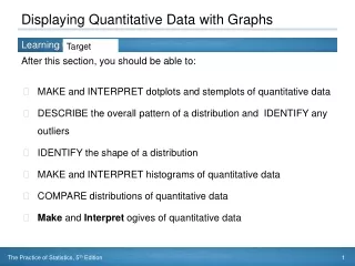
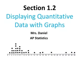
Displaying Quantitative Variables HistogramsThe most common graph for distribution of one quantitative variable.No spaces between groups.
How to construct a histogram 1. Divide range of data into classes of equal width and count number of observations in each class; be sure to specify classes precisely so that each observation falls into exactly one class. 2. Label and scale axis and title graph! 3. Draw a bar that represents the count in each class.
Remember: • Leave no space between bars. • Add a break-in-scale symbol (//) on an axis that does not start at 0. • 5 classes is a good minimum. • Histogram Tips (page 39)
Example Drive Time Professor Moore, who lives a few miles outside a college town, records the time he takes to drive to the college each morning. You previously entered the times (in minutes) into a list name “DRVTM” (pg.46, ex. 55) for the 42 consecutive weekdays, with the dates in order along the rows.
. a. Fill in freq. column and construct histogram. Drivetime Frequency 6.5-7.0 1 7.0-7.5 2 7.5 -8.0 8 8.0-8.5 11 8.5-9.0 12 9.0-9.5 6 9.5-10.0 1 10.0-10.5 1
Is the distribution roughly symmetric, clearly skewed, or neither? Are there any clear outliers? The distribution is roughly symmetric with no clear outliers. • B. Graph (Note: Your graph needs to be specific)
c. Make a calculator histogram of these drive times. Make calculator histogram and use the trace key. • STATPLOT:Plot1:On • Xlist:2ndSTAT:DRVTM:ENTER • Freq:1 (sometimes need to press ALPHA 1) • Window • Xmin=6, Xmax=11, Xscl=.5, ymin=0, ymax=13, yscl=1,xres=1 • Use the following classes and determine frequencies. • Can use Technology Toolbox as reference(p.38) • Used throughout the book to guide you step by step through various calculator functionalities.
Using Histograms Wisely • Don’t confuse histograms with bar graphs. • Bar Graph: ____________, compares the distribution of ______________. • Histograms: ______________, the distribution of ______________________.
Don’t use counts (freq) or percents (relative freq) as data. Length: 1 2 3 4 5 6 7 8 9 10 11 12 13 Count: 1 15 25 7 5 7 8 7 7 6 8 3 1 Graphed Incorrectly Draw Graph Correctly
Use percentsinstead of counts on the vertical axis when comparing distributions with different numbers of observations. Mary compared the number of letters in the first 200 words of a medical journal and of the first 100 words of an article from an airline magazine.