Download
1 / 5
60 likes | 227 Views
An Interactive session. lxplus> athena.py –i AnalysisSkeleton_jobOptions.py –l FATAL athena> include ("PyAnalysisCore/InitPyAnalysisCore.py") athena> theApp.initialize() initialization athena> theApp.algorithms() list all algorithms

E N D
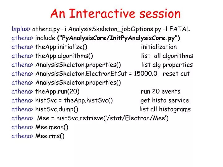
An Interactive session lxplus> athena.py –i AnalysisSkeleton_jobOptions.py –l FATAL athena> include ("PyAnalysisCore/InitPyAnalysisCore.py") athena> theApp.initialize() initialization athena> theApp.algorithms() list all algorithms athena> AnalysisSkeleton.properties() list alg properties athena> AnalysisSkeleton.ElectronEtCut = 15000.0 reset cut athena> AnalysisSkeleton.properties() athena> theApp.run(20) run 20 events athena> histSvc = theApp.histSvc() get histo service athena> histSvc.dump() list all histograms athena> Mee = histSvc.retrieve(‘/stat/Electron/Mee’) athena> Mee.mean() athena> Mee.rms()
An Interactive session-continue athena> from AidaProxy import * athena> from rootPlotter2 import * athena> plotter = RootPlotter() athena> plotter.plot (Mee) athena>plot(“ParticleJetContainer#ParticleJetContainer","$x.pt()",nEvent=5) athena> ntupleSvc = theApp.ntupleSvc() Athena> … (do not try the Fitter yet: it has some problem – I will inform you when it is fixed) athena> fitter = Fitter("Chi2","lcg_minuit") athena> fitParams = std.vector(double)() athena> fitParams.push_back(150.0) athena> fitParams.push_back(80000.0) athena> fitParams.push_back(5000.0)
An Interactive Session-continue athena> gaussian = Function(“G”) athena> gaussian.setParameters(fitParams) athena> fitResult = fitter.fit(Mee,gaussian) athena> if fitResult == None: athena> raise “Single gaussian chi2 fit failed” athena> parameterNames = fitResult.fittedParameterNames() athena>parameters = fitResult.fittedParameters() athena> errors = fitResult.errors() athena>for i in range(0,len(par)): athena> print parameterNames[i] + " = " + str(parameters[i]) + " +/- " + str(errors[i]) athena> plotter.plot(gaussion, “S”) Athena> … athena> theApp.exit() lxplus>
An Interactive Session - continue • You can put your interactive commands in a file and execute it on the Athena prompt • The file MyAnalysis.py contains: from AidaProxy import * from rootPlotter2 import * Import ROOT theApp.initialize() • Then, on the interactive ATHENA prompt: athena> execfile (“MyAnalysis.py”)
An Interactive Session - continue • It is recommended that you start your analysis an ATHENA algorithm such as the AnalysisSkeleton, where you implement some pre-defined histograms and NTuples • In an interactive session, you can access those histograms and NTuples. Further, you can also defined and fill new histograms on the fly • It is also possible to call C++ class from the ATHENA prompt • In an interactive session, you still have access to the full ROOT machinery through PyROOT.