Download
1 / 37
410 likes | 873 Views
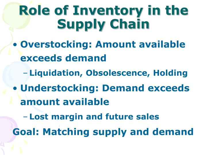
Role of Inventory in the Supply Chain. Overstocking: Amount available exceeds demand Liquidation, Obsolescence, Holding Understocking: Demand exceeds amount available Lost margin and future sales Goal: Matching supply and demand. Understanding Inventory. The inventory policy is affected by:

E N D
Role of Inventory in the Supply Chain • Overstocking: Amount available exceeds demand • Liquidation, Obsolescence, Holding • Understocking: Demand exceeds amount available • Lost margin and future sales Goal: Matching supply and demand
Understanding Inventory • The inventory policy is affected by: • Demand Characteristics • Lead Time • Number of Products • Objectives • Service level • Minimize costs • Cost Structure
Cost Structure • Order costs • Fixed • Variable • Holding Costs • Insurance • Maintenance and Handling • Taxes • Opportunity Costs • Obsolescence
EOQ: A View of Inventory* Note: • No Stockouts • Order when no inventory • Order Size determines policy Inventory Avg. Inventory Order Size Time
EOQ:Total Cost* Total Cost Holding Cost Order Cost
EOQ: Calculating Total Cost* • Purchase Cost Constant • Holding Cost: (Avg. Inven) * (Holding Cost) • Ordering (Setup Cost): Number of Orders * Order Cost • Goal: Find the Order Quantity that Minimizes These Costs:
Fixed costs: Optimal Lot Size and Reorder Interval (EOQ) R: Annual demand S: Setup or Order Cost C: Cost per unit h: Holding cost per year as a fraction of product cost H: Holding cost per unit per year Q: Lot Size T: Reorder interval
Example Demand, R = 12,000 computers per year Unit cost, C = $500 Holding cost, h = 0.2 Fixed cost, S = $4,000/order Q = 980 computers Cycle inventory = Q/2 = 490 Flow time = Q/2R = 0.49 month Reorder interval, T = 0.98 month
EOQ: Another Example • Book Store Mug Sales • Demand is constant, at 20 units a week • Fixed order cost of $12.00, no lead time • Holding cost of 25% of inventory value annually • Mugs cost $1.00, sell for $5.00 • Question • How many, when to order?
EOQ: Important Observations* • Tradeoff between set-up costs and holding costs when determining order quantity. In fact, we order so that these costs are equal per unit time • Total Cost is not particularly sensitive to the optimal order quantity
The Effect of Demand Uncertainty • Most companies treat the world as if it were predictable: • Production and inventory planning are based on forecasts of demand made far in advance of the selling season • Companies are aware of demand uncertainty when they create a forecast, but they design their planning process as if the forecast truly represents reality • Recent technological advances have increased the level of demand uncertainty: • Short product life cycles • Increasing product variety
Example: SnowTime Sporting Goods • Fashion items have short life cycles, high variety of competitors • SnowTime Sporting Goods • New designs are completed • One production opportunity • Based on past sales, knowledge of the industry, and economic conditions, the marketing department has a probabilistic forecast • The forecast averages about 13,000, but there is a chance that demand will be greater or less than this.
SnowTime Costs • Production cost per unit (C): $80 • Selling price per unit (S): $125 • Salvage value per unit (V): $20 • Fixed production cost (F): $100,000 • Q is production quantity, D demand • Profit = Revenue - Variable Cost - Fixed Cost + Salvage
SnowTime Scenarios • Scenario One: • Suppose you make 12,000 jackets and demand ends up being 13,000 jackets. • Profit = 125(12,000) - 80(12,000) - 100,000 = $440,000 • Scenario Two: • Suppose you make 12,000 jackets and demand ends up being 11,000 jackets. • Profit = 125(11,000) - 80(12,000) - 100,000 + 20(1000) = $ 335,000
SnowTime Best Solution • Find order quantity that maximizes weighted average profit. • Question: Will this quantity be less than, equal to, or greater than average demand?
(s, S) Policies • For some starting inventory levels, it is better to not start production • If we start, we always produce to the same level • Thus, we use an (s,S) policy. If the inventory level is below s, we produce up to S. • s is the reorder point, and S is the order-up-to level • The difference between the two levels is driven by the fixed costs associated with ordering, transportation, or manufacturing
Notation • AVG = average daily demand • STD = standard deviation of daily demand • LT = replenishment lead time in days • h = holding cost of one unit for one day • SL = service level (for example, 95%). This implies that the probability of stocking out is 100%-SL (for example, 5%) • Also, the Inventory Position at any time is the actual inventory plus items already ordered, but not yet delivered.
Analysis • The reorder point has two components: • To account for average demand during lead time:LTAVG • To account for deviations from average (we call this safety stock) z STD LTwhere z is chosen from statistical tables to ensure that the probability of stockouts during leadtime is100%-SL.
Example • The distributor has historically observed weekly demand of: AVG = 44.6 ; STD = 32.1Replenishment lead time is 2 weeks, and desired service level SL = 97% • Average demand during lead time is: 44.6 2 = 89.2 • Safety Stock is:1.88 32.1 2 = 85.3 • Reorder point is thus 175, or about 3.9 weeks of supply at warehouse and in the pipeline
Model Two: Fixed Costs* • In addition to previous costs, a fixed cost K is paid every time an order is placed. • We have seen that this motivates an (s,S) policy, where reorder point and order quantity are different. • The reorder point will be the same as the previous model, in order to meet meet the service requirement: s = LTAVG + z AVG L • What about the order up to level?
Model Two: The Order-Up-To Level* • We have used the EOQ model to balance fixed, variable costs:Q=(2 K AVG)/h • If there was no variability in demand, we would order Q when inventory level was at LT AVG. Why? • There is variability, so we need safety stockz AVG * LT • The total order-up-to level is: S=max{Q, [LT AVG+ z AVG * LT]}
Model Two: Example* • Consider the previous example, but with the following additional info: • fixed cost of $4500 when an order is placed • $250 product cost • holding cost 18% of product • Weekly holding cost:h = (.18 250) / 52 = 0.87 • Order quantityQ=(2 4500 44.6 / 0.87 = 679 • Order-up-to level:s + Q = 85 + 679 = 765
What to Make? • Question: Will this quantity be less than, equal to, or greater than average demand? • Average demand is 13,100 • Look at marginal cost Vs. marginal profit • if extra jacket sold, profit is 125-80 = 45 • if not sold, cost is 80-20 = 60 • So we will make less than average
SnowTime:Important Observations • Tradeoff between ordering enough to meet demand and ordering too much • Several quantities have the same average profit • Average profit does not tell the whole story • Question: 9000 and 16000 units lead to about the same average profit, so which do we prefer?
Key Points from this Model • The optimal order quantity is not necessarily equal to average forecast demand • The optimal quantity depends on the relationship between marginal profit and marginal cost • As order quantity increases, average profit first increases and then decreases • As production quantity increases, risk increases. In other words, the probability of large gains and of large losses increases
Initial Inventory • Suppose that one of the jacket designs is a model produced last year. • Some inventory is left from last year • Assume the same demand pattern as before • If only old inventory is sold, no setup cost • Question: If there are 7000 units remaining, what should SnowTime do? What should they do if there are 10,000 remaining?
Periodic Review Policy • Each review echelon, inventory position is raised to the base-stock level. • The base-stock level includes two components: • Average demand during r+L days (the time until the next order arrives):(r+L)*AVG • Safety stock during that time:z*STD* r+L
Inventory Management: Best Practice • Periodic inventory review policy (59%) • Tight management of usage rates, lead times and safety stock (46%) • ABC approach (37%) • Reduced safety stock levels (34%) • Shift more inventory, or inventory ownership, to suppliers (31%) • Quantitative approaches (33%)
Inventory Management: Best Practice • Periodic inventory reviews • Tight management of usage rates, lead times and safety stock • ABC approach • Reduced safety stock levels • Shift more inventory, or inventory ownership, to suppliers • Quantitative approaches
Changes In Inventory Turnover • Inventory turnover ratio = annual sales/avg. inventory level • Inventory turns increased by 30% from 1995 to 1998 • Inventory turns increased by 27% from 1998 to 2000 • Overall the increase is from 8.0 turns per year to over 13 per year over a five year period ending in year 2000.
Factors that Drive Reduction in Inventory • Top management emphasis on inventory reduction (19%) • Reduce the Number of SKUs in the warehouse (10%) • Improved forecasting (7%) • Use of sophisticated inventory management software (6%) • Coordination among supply chain members (6%) • Other
Factors that Drive Inventory Turns Increase • Better software for inventory management (16.2%) • Reduced lead time (15%) • Improved forecasting (10.7%) • Application of SCM principals (9.6%) • More attention to inventory management (6.6%) • Reduction in SKU (5.1%) • Others