Generalized Dynamical Mean - Field Theory for Strongly Correlated Systems

1. E.Z.Kuchinskii1, I.A. Nekrasov1, M.V.Sadovskii1,2 Generalized Dynamical Mean - Field Theory for Strongly Correlated Systems 1Institute for Electrophysics and 2Instutute for Metal Physics , Russian Academy of Sciences, Ekaterinburg, Russia

3. Hubbard model J.Hubbard (1964) Correlated Metal Mott Insulator

4. Traditional DMFT approach J.Hubbard (1964) In the limit of spatial dimensionality self - energy becomes local, i.e. Then the problem can be exactly (!) mapped on the equvalent problem of Anderson impurity, which is to be solved by some kind of “impurity solver” (QMC, CTQMC, NRG, NCA etc.) W.Metzner, D.Vollhardt, 1989, A.Georges, G.Kotliar, 1992, Th.Pruschke, M.Jarrell, 1992 The absence of k - dependence of electron self - energy is the basic shortcoming of the traditional DMFT, however only due to this fact we obtain an exact solution!

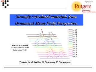
5. Numerical Results N Standard DMFT results demonstrate formation of Hubbard bands and quasiparticle (Fermi - liquid) band at the Fermi level. W=2D=2Zt=4 Uc=1.5W=6 Energies here in units of t for Z=4(square lattice) Metal - insulator transition atU=6. Critical point Mott Insulator Metal

6. Basics of DMFT+ approach M.V.Sadovskii, I.A.Nekrasov, E.Z.Kuchinskii, Th.Pruschke, V.I.Anisimov (2005) • DMFT+: k - self-energy due to any “external” interaction!

7. DMFT+calculation scheme:

9. Electron – phonon interaction and “kinks” • Electron – phonon interactionleads toa “kink”in electron dispersionwithin energy interval of2ħD around the Fermi level. • Electron velocity:(A.B. Migdal, 1957) • v(k)=1/ħ·ek /k=v0(k)/(1+l), • Effective mass renormalization: • m*/m=1+l • – dimensionles electron–phonon coupling “Kinks” are now well observed in ARPES “

10. “Kinks” - Experimental ARPESdirectly measures electron spectral densitywhich allows to determine quasiparticle dispersion ~40-70 мэВ For HTSC cuprates“kink” energy ~ 40-70 meV, TD~400-700K Sato et al., PRL 91, 157003 (2004)

11. “Electronic kinks” in Hubbard model: DMFT K.Byczuk et al. Nature Phys. 3, 168 () K.Buczuk, I.A.Nekrasov, D.Vollhardt et al. (2007) “Kink” energy Fermi – liquid renormalization:

12. DMFT+k for Electron – Phonon Interaction Dph DMFT self-energy Electron – phonon self-energy + Migdal theorem – el-ph vertexcorrections small as xp – free (band) electrons

13. DMFT+: “Kinks” in Electron Dispersion Different “geometries” of “kinks” due to electron-phohon interaction and correlations

14. DMFT+: Self-energy and Dispersion M.V.Sadovskii, I.A.Nekrasov,E.Z.Kuchinskii (2009) “Kinks” coexist if:

15. Dependence of electron – phonon “kink” onU M.V.Sadovskii, I.A.Nekrasov,E.Z.Kuchinskii (2006) Quasiparticle dispersions around Fermi level with phonon kinks obtainedfrom DMFT+ calculations for different interaction strengths: U/2D= 0.5, 0.75, 1.0;  = 0.8; D=0.1D.

16. Disorder Induced Metal-Insulator Transition Anderson model P.W.Anderson (1958)

17. Anderson - Hubbard Model

18. Self-consistent Born approximation for impurity scattering Semi - elliptic DOS:

19. Dynamic conductivity in DMFT+ M.V.Sadovskii, I.A.Nekrasov, E.Z.Kuchinskii (2006)

20. Dynamic (optical) conductivity  DMFT+!   q 2    

21. General expression for dynamic conductivity in DMFT+: No Hubbard U in vertices here! M.V.Sadovskii, I.A.Nekrasov,E.Z.Kuchinskii (2006)

22. Density of States (d=3)

23. Conductivity and Metal-Insulator Transition (d=3)

24. Phase Diagram (d=3) M.V.Sadovskii, I.A.Nekrasov,E.Z.Kuchinskii (2006 - 2012) Calculated in DMFT+

25. Pseudogap in Cuprates J.Campuzano et al. (2004) M.Norman et al. (1998)

27. Pseudogaps and “Hot - Spots” model x w - frequency of fluctuations - correlation length sf D.Pines et al. SF-model (1990 - 1999) J.Campuzano et al. (2004) Eg ~ D J.Loram, J.Tallon (2001) NdCeCuO - N.Armitage et al. (2001)

28. Sk for AFM (CDW) fluctuations We take into account ALL(!) diagrams for quenched (Gaussian) AFM (CDW) fluctuations M.V.Sadovskii, 1979 E.Z.Kuchinskii, M.V.Sadovskii, 1999 D.Pines, J.Schmalian, B.Stoikovic,1999 Valid forT>>wsf ! Spin - Fermion (SF) or CDW model S(n) - is defined by diagram combinatorics (AFM(SDW), CDW, commensurate etc.)

29. Densities of states - correlated metal(U<W) t’=- 0.4t t’=0 DMFT+k results Impuruty solver -NRG K.G.Wilson, 1975, R.Bulla, A.C.Hewson, Th. Pruschke, 1999

30. Spectral densities and ARPES Typical Fermi surface of copper - oxide superconductor (La2-xSrxCuO4) Z.X.Shen et al. (2004) M G X

33. “Destruction” of the Fermi surface M.V.Sadovskii, I.A.Nekrasov,E.Z.Kuchinskii (2005)

34. ARPES Fermi surface - (Bi,Pb)2212, NCCO A.Kordyuk, S.Borisenko, J.Fink et al. (2002)

35. ARPES and LDA+DMFT+S:

36. Two-particleproperties and Linear Response Recursion relations for effective vertex - interaction with pseudogap fluctuations. M.V.Sadovskii, N.A.Strigina (2002) M.V.Sadovskii, I.A.Nekrasov,E.Z.Kuchinskii (2007)

37. DMFT+S optical conductivity in strongly correlated metal Conductivity in units of

38. Optical evidence for pseudogaps in oxides Bi2212 Y.Onose et al. (2003) 123 J.Loram, J.Tallon et al. (1997) T.Startseva et al. (1999) T.Timusk et al. (2006)

39. Single band sum rule: This should be valid in any reasonable model of optical conductivity! Dependence of the r.h.s. on temperature and any other parameter is sometimes called “sum rule violation”. V.

40. Check of the general optical sum rule (d=3): /2D W SR 0 0,063 0,064 0,25 0,068 0.07 0,37 0,06 0.061 0,43 0,056 0.056 0,50 0,049 0.05

41. Conclusions: • DMFT+S - universal and effective way to include “external” interactions to DMFT • DMFT+S - effective way to take into account nonlocal corrections to DMFT • DMFT+S can be easily generalized for “realistic” calculations (LDA+DMFT+S) • Many applications already demonstrated the effectiveness of DMFT+S, more to come • Review: E.Z.Kuchinskii, I.A.Nekrasov, M.V.Sadovskii. Physics Uspekhi 55, No.4. (2012); ArXiv: 1109.2305; УФН 182, No.4, 345-378 (2012) ET