Download
1 / 58
770 likes | 1.3k Views
Chapter 4 Experiments with Blocking Factors. 4.1 The Randomized Complete Block Design. Nuisance factor: a design factor that probably has an effect on the response, but we are not interested in that factor.

E N D
4.1 The Randomized Complete Block Design • Nuisance factor: a design factor that probably has an effect on the response, but we are not interested in that factor. • Typical nuisance factors include batches of raw material, operators, pieces of test equipment, time (shifts, days, etc.), different experimental units
If the nuisance variable is known and controllable, we use blocking • If the nuisance factor is known and uncontrollable, sometimes we can use the analysis of covariance (see Chapter 14) to remove the effect of the nuisance factor from the analysis
If the nuisance factor is unknown and uncontrollable (a “lurking” variable), we hope that randomization balances out its impact across the experiment • Sometimes several sources of variability are combined in a block, so the block becomes an aggregate variable
We wish to determine whether 4 different tips produce different (mean) hardness reading on a Rockwell hardness tester • Assignment of the tips to an experimental unit; that is, a test coupon • Structure of a completely randomized experiment • The test coupons are a source of nuisance variability • Alternatively, the experimenter may want to test the tips across coupons of various hardness levels • The need for blocking • Randomized Complete block design (RCBD)
To conduct this experiment as a RCBD, assign all 4 tips to each coupon • Each coupon is called a “block”; that is, it’s a more homogenous experimental unit on which to test the tips • Variability between blocks can be large, variability within a block should be relatively small • In general, a block is a specific level of the nuisance factor • A complete replicate of the basic experiment is conducted in each block • A block represents a restriction on randomization • All runs within a block are randomized
Suppose that we use b = 4 blocks: • Once again, we are interested in testing the equality of treatment means, but now we have to remove the variability associated with the nuisance factor (the blocks)
Statistical Analysis of the RCBD • Suppose that there are a treatments (factor levels) and b blocks • A statistical model (effects model) for the RCBD is • is an overall mean, i is the effect of the ith treatment, and j is the effect of the jth block • ij ~ NID(0,2)
Means model for the RCBD • The relevant (fixed effects) hypotheses are • An equivalent way for the above hypothesis • Notations:
SST = SSTreatment + SSBlocks + SSE • Total N = ab observations, SST has N – 1 degrees of freedom. • a treatments and b blocks, SSTreatmentand SSBlocks have a – 1 and b – 1 degrees of freedom. • SSE has ab – 1 – (a – 1) – (b – 1) = (a – 1)(b – 1) degrees of freedom. • From Theorem 3.1, SSTreatment /2, SSBlocks / 2and SSE / 2 are independently chi-square distributions.
The expected values of mean squares: • For testing the equality of treatment means,
The ANOVA table • Another computing formulas:
To conduct this experiment as a RCBD, assign all 4 pressures to each of the 6 batches of resin • Each batch of resin is called a “block”; that is, it’s a more homogenous experimental unit on which to test the extrusion pressures
4.1.2 Model Adequacy Checking • Residual Analysis • Residual: • Basic residual plots indicate that normality, constant variance assumptions are satisfied • No obvious problems with randomization
Can also plot residuals versus the type of tip (residuals by factor) and versus the blocks. Also plot residuals v.s. the fitted values. • These plots provide more information about the constant variance assumption, possible outliers 4.1.3 Some Other Aspects of the Randomized Complete Block Design • The model for RCBD is complete additive.
Interactions? • For example: • The treatments and blocks are random. • Choice of sample size: • Number of blocks , the number of replicates and the number of error degrees of freedom
Estimating miss values: • Approximate analysis: estimate the missing values and then do ANOVA. • Assume the missing value is x. Minimize SSE to find x • The error degrees of freedom - 1
4.1.4 Estimating Model Parameters and the General Regression Significance Test • The linear statistical model • The normal equations
Under the constraints, the solution is and the fitted values, • The sum of squares for fitting the full model: • The error sum of squares
4.2 The Latin Square Design • RCBD removes a known and controllable nuisance variable. • Example: the effects of five different formulations of a rocket propellant used in aircrew escape systems on the observed burning rate. • Remove two nuisance factors: batches of raw material and operators • Latin square design: rows and columns are orthogonal to treatments.
The Latin square design is used to eliminate two nuisance sources, and allows blocking in two directions (rows and columns) • Usually Latin Square is a p p squares, and each cell contains one of the p letters that corresponds to the treatments, and each letter occurs once and only once in each row and column. • See Page 139
The statistical (effects) model is • yijk is the observation in the ith row and kth column for the jth treatment, is the overall mean, i is the ith row effect, jis the jth treatment effect, k is the kth column effect and ijkis the random error. • This model is completely additive. • Only two of three subscripts are needed to denote a particular observation.
Sum of squares: SST = SSRows + SSColumns + SSTreatments + SSE • The degrees of freedom: p2 – 1 = p – 1 + p – 1 + p – 1 + (p – 2)(p – 1) • The appropriate statistic for testing for no differences in treatment means is • ANOVA table
least squares estimates of the model parameters, i , j , k
The residuals • If one observation is missing,
Standard Latin square • Random order
Replication of Latin Squares: • The same batches and operators
Replication of Latin Squares: • The same batches and different operators
Replication of Latin Squares: • The different batches and different operators
4.3 The Graeco-Latin Square Design • Graeco-Latin square: • Two Latin Squares • One is Greek letter and the other is Latin letter. • Two Latin Squares are orthogonal • Table 4.17 • Block in three directions • Four factors (row, column, Latin letter and Greek letter) • Each factor has p levels. Total p2runs
The statistical model: • yijkl is the observation in the ith row and lth column for Latin letter j, and Greek letter k • is the overall mean, i is the ith row effect, j is the effect of Latin letter treatment j , k is the effect of Greek letter treatment k, l is the effect of column l. • ANOVA table (Table 4.18) • Under H0, the testing statistic is Fp-1,(p-3)(p-1) distribution.
Example 4.4 • Add a block factor: 5 test assemblies
4.4 Balance Incomplete Block Designs • May not run all the treatment combinations in each block. • Randomized incomplete block design (BIBD) • Any two treatments appear together an equal number of times. • There are a treatments and each block can hold exactly k (k < a) treatments. • For example: A chemical process is a function of the type of catalyst employed.
4.4.1 Statistical Analysis of the BIBD • a treatments and b blocks. Each block contains k treatments, and each treatment occurs r times. There are N = ar = bk total observations. The number of times each pairs of treatments appears in the same block is • The statistical model for the BIBD is