Download
1 / 26
260 likes | 421 Views
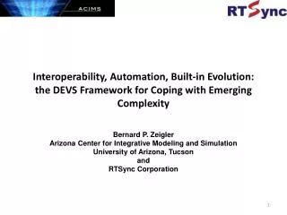
Continuity and Change (Activity) Are Fundamentally Related In DEVS Simulation of Continuous Systems Bernard P. Zeigler. Arizona Center for Integrative Modeling and Simulation (ACIMS) University of Arizona Tucson, Arizona 85721, USA zeigler@ece.arizona.edu www.acims.arizona.edu. Outline.

E N D
Continuity and Change (Activity) Are Fundamentally Related In DEVS Simulation of Continuous SystemsBernard P. Zeigler Arizona Center for Integrative Modeling and Simulation(ACIMS) University of ArizonaTucson, Arizona 85721, USAzeigler@ece.arizona.eduwww.acims.arizona.edu
Outline • Review DEVS Framework for M&S • Brief History of Activity Concept Development • Summary of Recent Results • Theory of Event Sets – Basis for Activity Theory • Conclusions and Implications
Synopsis • A continuous curve can be represented by a sequence of finite events sets whose points get closer together at just the right rate • We can measure the amount of change in such a continuous curve – this is its activity • The activity divided by the largest change in an event set gives the size of this set’s most economical representation • DEVS quantization can achieve this optimal representation
DEVS Background • DEVS = Discrete Event System Specification • Based on formal M&S framework • Derived from mathematical dynamical system theory • Supports hierarchical, modular composition • Object oriented implementation • Supports discrete and continuous paradigms • Exploits efficient parallel and distributed simulation techniques
DEVS Hierarchical Modular Composition Atomic: lowest level model, contains structural dynamics -- model level modularity Coupled: composed of one or more atomic and/or coupled models Hierarchical construction + coupling
DEVS Theoretical Properties • Closure Under Coupling • Universality for Discrete Event Systems • Representation of Continuous Systems • quantization integrator approximation • pulse representation of wave equations • Simulator Correctness, Efficiency
DEVS Expressability Coupled Models Atomic Models Partial Differential Equations can be components in a coupled model Ordinary Differential Equation Models Processing/ Queuing/ Coordinating Networks, Collaborations Physical Space Spiking Neuron Networks Spiking Neuron Models Processing Networks Petri Net Models n-Dim Cell Space Discrete Time/ StateChart Models Stochastic Models Cellular Automata Quantized Integrator Models Self Organized Criticality Models Fuzzy Logic Models Reactive Agent Models Multi Agent Systems
Activity Theory unifies continuous and discrete paradigms DEVS can represents all decision making and continuous dynamic elements Heterogeneous activity in time and space Quantization allows DEVS to naturally focus computing resources on high activity regions DEVS concentrates its computational resources at the regions of high activity. While DEVS uses smaller time advance (similar to time step in DTSS) in regions of high activity. DTSS uses the same time step regardless of the activity.
s d s /dt s ò 1 1 x x f 1 s d s /dt s ò 2 2 x f 2 ... s d s /dt s ò n n x f n s d s /dt s F ò 1 1 DEVS x x f 1 S s d s /dt s DEVS ò 2 2 x f F 2 ... s d s /dt s ò DEVS F n n x f n Mapping Ordinary Differential Equation Systems into DEVS Quantized Integration DEVS Integrator DEVS instantaneous function Theory of Modeling and Simulation, 2nd Edition, Bernard P. Zeigler , Herbert Praehofer , Tag Gon Kim ,Academic Press, 2000.
PDE Stability Requirements • Courant Condition requires smaller time step for smaller grid spacing for partial differential equation solution • This is a necessary stability condition for discrete time methods but not for quantized state methods Ernesto Kofman, Discrete Event Based Simulation and Control of Hybrid Systems, Ph.D. Dissertation: Faculty of Exact Sciences, National University of Rosario, Argentina
Activity – a characteristic of continuous functions b #Threshold Crossings = Activity/quantum a Activity = |b-a| Activity(0,T) =
#DEVS Transitions = #Threshold Crossings R. Jammalamadaka,, Activity Characterization of Spatial Models: Application to the Discrete Event Solution of Partial Differential Equations, M.S. Thesis: Fall 2003, Electrical and Computer Engineering Dept., University of Arizona
H B H/2 A 0 N-1 (N-1)/2 L H A HW/L B 0 W L Activity Calculations for 1-D Diffusion This shows that the activity per cell in all the three cases goes to a constant as N (number of cells) tends to infinity.
DEVS Efficiency Advantage where Activity is Heterogeneous in Time and Space activity A # crossings =A/q Potential Speed Up = #time steps / # crossings quantum q X time step size number of cells # time steps =T/ Time Period T
#DTSS/#DEVS Ratio for 1-D Diffusion *f is an increasing function of L Alexander Muzy’s scalability results
Muzy’s Fire Front model Accumulated Activity Instantaneous Activity Region Of Imminence Peak Bars S. R. Akerkar, Analysis and Visualization of Time-varying data using the concept of 'Activity Modeling', M.S. Thesis, University of Arizona,2004
DEVS vs DTSS in Parallel Distributed Simulation J. Nutaro, Parallel Discrete Event Simulation with Application to Continuous Systems, Ph. D. Dissertation Fall 2003,, Univerisity of Arizona
QFFT Module 1 1 1 1 2 2 2 2 3 3 3 3 4 4 4 4 . . . . . . . . . . . . . . . . . . . . . . . . . . . N/2 Units N/2 Units N/2 Units N-1 N-1 N-1 N-1 N N N N q = q0/N q = q0/(N-1) q = q0/1 Q Q Q Q Q Q Q Q Q B B B B B B B B B n = log2N Stages Q = Quantizer B = Butterfly N = 1024 (powers of 2) n = 10 (log2N) q = Quantum for respective stage Quantization in Digital Processing Transmit to next stage only when quantum exceeded Harsha Gopalakrishnan, DEVS Scalable Modeling of a High performance pipelined DIF FFT core with Quantization, MS Thesis U. Arizona.
QFFT System Output QFFT Module (Backward Transform) Analog LPF 3000 Hz cut-off QFFT Module (Forward Transform) Input 300 – 3000 Hz Voice 300 Hz - 3000 Hz At q = .06 Music 300 Hz - 3000 Hz At q = .02 Reduction (at q0 = 0.06) = 52% Reduction (at q0 = 0.02) = 30.8%
size = 5 size = 9 size = 17 size = 33 Event set refinement sequence
Domain and Range Based Event Sets domain-based event set with equally spaced domain points separated by step denote a range-based event set with equally spaced range values, separated by a quantum . For an n-th degree polynomial we have . So that potential gains of the order of are possible.
Conclusions • Activity Theory confirms that where there is heterogeneity of activity in space and time, DEVS will have significant advantage over conventional numerical methods • This lead us to try reformulating the math foundations of continuity in discrete event terms
Implications • sensing– most sensors are currently driven at high sampling rates to obviate missing critical events. Quantization-based approaches require less energy and produce less irrelevant data. • data compression – even though data might be produced by fixed interval sampling, it can be quantized and communicated with less bandwidth by employing domain-based to range-based mapping. • reduced communication in multi-stage computations, e.g., in digital filters and fuzzy logic is possible using quantized inter-stage coupling. • spatial continuity–quantization of state variables saves computation and our theory provides a test for the smallest quantum size needed in the time domain; a similar approach can be taken in space to determine the smallest cell size needed, namely, when further resolution does not materially affect the observed spatial form factor. • coherence detection in organizations – formations of large numbers of entities such as robotic collectives, ants, etc. can be judged for coherence and maintenance of coherence over time using this paper’s variation measures. • education -- revamp teach of the calculus to dispense with its mysterious foundations (limits, continuity) that are too difficult to convey to learners.