Download
1 / 87
890 likes | 1.12k Views
Model Selection for SVM & Our intent works. Songcan Chen Feb. 8, 2012. Outline. Model Selection for SVM Our intent works. Model Selection for SVM. Introduction to 2 works. Introduction to 2 works. Model selection for primal SVM [MBB11, MLJ11] Selection of Hypothesis Space

E N D
Model Selection for SVM&Our intent works Songcan Chen Feb. 8, 2012
Outline • Model Selection for SVM • Our intent works
Model Selection for SVM • Introduction to 2 works
Introduction to 2 works • Model selection for primal SVM[MBB11, MLJ11] • Selection of Hypothesis Space • Selecting the Hypothesis Space for Improving the Generalization Ability of Support Vector Machines[AGOR11,IJCNN2011] • The Impact of Unlabeled Patterns in Rademacher Complexity Theory for Kernel Classifiers [AGOR11,NIPS2011]
1st work • Model selection for primal SVM [MBB11, MLJ11] [MBB11] Gregory Moore · Charles Bergeron · Kristin P. Bennett, Machine Learning (2011) 85:175–208
Outline • Primal SVM • Model selection 1) Bilevel Program for CV 2) Two optimization Methods: Impilicit & Explicit methods 3) Experiments 4) Conclusions
Primal SVM • Advantages: 1) simple to implement, theoretically sound, and easy to customize to different tasks such as classification, regression, ranking and so forth. 2) very fast, linear in the number of samples • Difficulty model selection
Model selection An often-adopted approach: Cross-validation (CV) over a grid Advantage: simple and almost universal! Weakness: high computation exponential in the number of hyperparameters and the number of grid points for each hyperparameter.
Motivation • CV is naturally and precisely formulated as a bilevel program (BP) shown as follows. Bilevel CV Problem (BCP)
Bilevel CV Problem (BCP) (1) BCP for a single validation and training split: • The outer-level leader problem selects the hyperparameters, γ, to perform well on avalidation set. • The follower problem trains an optimal inner-level model for the given hyperparameters, and returns a weightvectorw for validation.
Bilevel CV Problem (BCP) (2) More Specifically, Model selection via T-fold CV BCP! • The inner-level problems minimize theregularized training error to determine the best function for the given hyperparameters for each fold. • The hyperparameters are the outer-level control variables. The objective of the outer-level is to minimize the validation error based on the optimal parameters (w) returned for each fold.
Formal Formulation for BCP (1) • Given a training sample Ω:= {xj, yj}, j=1… l∈ Rn+1. • T-CV: PartitionΩ into T equally sized divisions; then for fold t=1…T, one of the divisions is used as the validation set, , and the remaining T-1 divisions are assigned to the training set, . • Letγ∈Rmbe the set of m model hyperparameters and wtbe the model weights for the t-th fold.
Formal Formulation for BCP (2) Let be the inner-level training function given the t-th fold training dataset and be the t-th outer-level validation loss function given its validation dataset
Formal Formulation for BCP (3) The bilevel program for T-fold CV is: (2) The BCP is challenging to solve in this form.
Formal Formulation for BCP (4) (3) Two solution methods: 1) Implicit and 2) explicit
Implicit method (1) i.e., make wan implicit function ofγ, namely w(γ). (4) Forming a nonlinear objective! In practice, nonlinear objectives are much easier to optimize than nonlinear constraints. Where w(γ)is computed such that
Implicit method (2) Since for optimality, Equivalently having the KKT condition (5)
Implicit method (3) • The reformulated BCP becomes: (6) (7)
One of Applications • Implicit Model selection for SVR • Objective of SVR(9) and optimality condition(10) are, respectively: (9) (10)
Defining the objective functions Lin and Lout for SVR respectively: First, each fold t in T-fold CV contributes a validation mean squared error: (11)
The T-folds are averaged to generate the outer-level objective: (12) For single group SVR, there are T inner-level objectives Lin: (13)
Implicit model selection for SVR (14) A full Bilevel Program (BP)
For multiple group SVR (multiSVR) 1) multiSVR’s objective: (15) 2) Optimality condition or constraint (16)
Implicit model selection methods:Algorithm (ImpGrad) where (17)
Summary for ImpGrad • ImpGrad alternates between training a model and updating the hyperparameters. Ideally an explicit algorithm that simultaneously solves for both model weights and hyperparameters would be more efficient as there is no need to train a model to optimality when far from the optimal solution.
Explicit Methods (1) Assume that the inner-level objective functions are differentiable and convex with respect to w, thus the optimality condition is the partial derivative of Lin(w, γ)with respect to wis equal to zero:
Explicit Methods (2) In position to transforming a bilevel program to the nonconvex nonsmooth program
PBP Algorithm (2) where (35)
One of Applications SVR using the PBP algorithm
The optimality condition to be penalized for each inner-level problem, t = 1 . . . T , is:
Experiments • Experiment A: Small QSAR datasets • Experiment B: Large QSAR datasets
Experiment B (2): MSE For Pyruvate kinase Dataset
Experiment B (3): MSE For Tau-fibril Dataset
Summary • Coarse grid search was reasonably fast; faster than both ImpGrad and PBP. In terms of generalization though, coarse grid search performed the worst. • Implicit and PBP algorithms performed better, with PBP being faster on the smaller datasets and ImpGrad being faster on the larger datasets. Generalization was slightly better for PBP.
Conclusions (1) • ImpGradfinds solutions with good generalization very quickly for large datasets, but illustrates more erratic behavior on all of the small datasets. • PBPuses a well-founded subgradient method with proven convergence properties and yields a robust explicit algorithm that performed well on problems of all sizes. While it appears to be roughly linear in the training time required per modeling set size.
Conclusions (2) • Like all machine learning algorithms, PBP and ImpGrad have algorithm parameters that must be defined such as exit criteria, starting points, and proximity parameters. • ImpGrad and PBP assume that the inner-level objective functions are at least once differentiable.