Download
1 / 36
530 likes | 1.09k Views
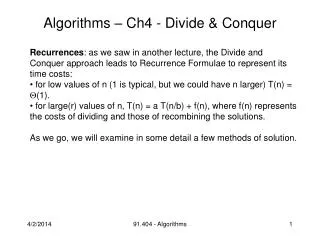
Divide and Conquer Algorithms. Algorithm design strategy: Divide and Conquer if the problem is small, solve directly if the problem is large, divide into two or more subproblems solve the smaller subproblems using the same divide-and-conquer approach

E N D
Divide and Conquer Algorithms • Algorithm design strategy: Divide and Conquer • if the problem is small, solve directly • if the problem is large, divide into two or more subproblems • solve the smaller subproblems using the same divide-and-conquer approach • combine the subproblem solutions to get a solution for the larger problem • Divide and Conquer algorithms are often implemented as recursive functions
Trominos and Deficient Boards • (Right) Tromino:object made up of three 11 squares that are not linearly arranged • Deficient board:A nn board of 11 squares with one square removed Three of the sixteen possible deficient 44 boards
A Tiling Problem • Tromino Tiling of a Deficient Board:An exact covering of all the squares of the board by non-overlapping trominos none of whom extend outside the board • Tromino Tiling Problem:Given a nn deficient board, where n is a power of 2, find a tiling of the board by trominos
Tiling Algorithm • Divide and Conquer algorithm for the tromino tiling problem: Small case: a deficient 22 board is a tromino, so we are done. Large case: n = 2k with k 2 Divide the board into four 2k-12k-1 boards, exactly one of which will be deficient. For each non-deficient quadrant, “remove” the square touching the center point of the original board Recursively tile the deficient quadrant Add the tromino made up of the squares not covered in the non-deficient quadrants.
Tiling Other Deficient Boards • A deficient nn board is made up of n2-1 squares • Since a tromino is made up of 3 squares, if a deficient nn board can be tiled by trominos, then n2-1 must be divisible by 3. • Thus n2-1 being divisible by 3 is a necessary condition for a tiling to exist • Chu and Johnsonbaugh proved that this condition is also sufficient for all n except n = 5. • There are deficient 55 boards that can be tiled and others that cannot.
Mergesort • Mergesort: a divide and conquer algorithm for sorting • Small cases: a single element array, which is already sorted • Large cases: • split the array into two “equal” size parts • recursively sort the two parts • merge the two sorted subarrays into a sorted array • The key to mergesort is the merge algorithm
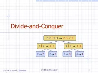
Mergesort • Merging two sorted arrays into an output array
Mergesort • Merging two sorted arrays into an output array • Start by examining the first elements of each array • Copy the smaller of the two into the output array
Mergesort • Merging two sorted arrays into an output array • Start by examining the first elements of each array • Copy the smaller of the two into the output array • Move to the right in the array from which the value was copied
Mergesort • Merging two sorted arrays into an output array • Start by examining the first elements of each array • Copy the smaller of the two into the output array • Move to the right in the array from which the value was copied • Copy the smaller of the two values into the output array
Mergesort • Merging two sorted arrays into an output array • Start by examining the first elements of each array • Copy the smaller of the two into the output array • Move to the right in the array from which the value was copied • If this is not possible, copy the remaining values from the other array into the output array
Mergesort • Merging two sorted arrays into an output array • Start by examining the first elements of each array • Copy the smaller of the two into the output array • Move to the right in the array from which the value was copied • If this is not possible, copy the remaining values from the other array into the output array
Merge Algorithm • Input parameters: array a, indices i, m, j • Output parameters: array a • Preconditions: a[i..m] is sorted and a[m+1..j] is sorted • Postcondition: a[i..j] is sorted merge(a,i,m,j) {
Merge Algorithm merge(a,i,m,j) { p = i // index in a[i .. m]q = m+1 // index in a[m+1 .. j]r = i // index in local array c while ( p m and q j ) { if (a[p] a[q] ) { c[r] = a[p] p = p+1 } else { c[r] = a[q] q = q+1 } r = r+1} // At this point one of the subarrays has been exhausted
Merge Algorithm // merge(a,i,m,j) continued // At this point one of the subarrays has been exhausted while (p m) { c[r] = a[p] p = p+1; r = r+1} while (q j) { c[r] = a[q] q = q+1; r = r+1} for( r = i to j) // copy c back to a a[r] = c[r] } Running time: (n)
Mergesort mergesort(a,i,j) { if ( i == j ) // only one element, so return return m = (i+j)/2 mergesort(a,i,m) mergesort(a,m+1,j) merge(a,i,m,j) } Recurrence for worst-case running time: T(n) = T(n/2) + T(n/2) + 2n T(n) 2T(n/2) + 2n, so by the Master Theorem, T(n) is O(nlg n) T(n) 2T(n/2) + 2n, so by the Master Theorem T(n) is (nlg n) T(n) is (nlg n)
Closest Pair of Points Problem • In this problem we have a collection of points in the plane and we wish to find the shortest distance between pairs of points in the collection: • Let P = { p1, p2, . . . , pn } be a collection of points in the plane • Thus we want to find min { dist(pi,pj) | 1 ≤ i < j ≤ n } • The following obvious algorithm will find the distance between a closest pair of points in P: min for i 1 to n-1 for j i+1 to n if dist(pi,pj) < min min = dist(pi,pj)return min • The running time of the above is clearly (n2) • Divide and Conquer can be used to get a (nlg n) algorithm
Closest Pairs Algorithm • First step (Divide) Choose a vertical line L so that n/2 of the points are on or to the left of L (left set) and n/2 points of P are on or to the right of L (right set) • Second step (Conquer) Recursively compute the minimum distance L between any two points in the left set of points and the minimum distance R between any two points in the right set of points. Let = min{ L, R } • Three possibilities: (1) a closest pair of points in P lie in the left set, giving L as the overall min (2) a closest pair of points in P lie in the right set, giving R as the overall min (3) a closest pair of points in P has one point in the left set and the other in the right set and this distance is less than
Closest Pairs Algorithm • First step (Divide) Choose a vertical line L so that n/2 of the points are on or to the left of L (left set) and n/2 points of P are on or to the right of L (right set)
Closest Pairs Algorithm • Thus we must check to see if there is a pair of points from different sides of L whose distance is less than • First observation: If p is a point in the either the left or right set whose x-coordinate differs by more than from the x-coordinate c of the vertical line L, then its distance to any point in the other set . Thus we need only consider points whose x-coordinate satisfies c- < x < c+ Thus we may reduce the set of points to be considered to those lying in the open vertical strip of width 2 centered at L
Closest Pairs Algorithm • Second observation: If we consider the points in the strip in order of non-decreasing y-coordinate, we need only compare each point with points above it Moreover, when checking point p, we need only consider points whose y-coordinate is less than more than that of p. This means that we only consider points in the rectangle with width 2 and height centered on the line L and having p on its lower edge
Closest Pairs Algorithm • Third observation: There are at most 7 other points in the rectangle for p Break the rectangle up into /2 by /2 squares: The distance between two points in /2 by /2 square is ≤ Since each square is contained in the left or the right set, it can containat most one of the points in P
Running Time • If we consider the points in the strip in non-decreasing order of their y-coordinates, we need only compare each point to at most 7 other points • Thus the cost of finding the smallest distance between pairs of points in the strip is at most 7n • This gives the following recurrence for the running time: T(n) = T(n/2 ) + T(n/2 ) + 7n • By the Master Theorem, we then have T(n) = (nlg n)
Closest Pair Algorithm closest_pair(p) { n = p.last mergesort(p,1,n) // sort by x-coordinate return recursive_closest_pair(p,1,n) } // recursive_closest_pair assumes that the input is sorted by x-coordinate // At termination, the input is stably sorted by y-coordinate
Closest Pair Algorithm recursive_closest_pair(p,i,j) { if (j-i < 3) { mergesort(p,i,j) // sort by y-coordinate // Find a closest pair directly delta = dist(p[i],p[i+1]) if (j-i = 1) // two pointsreturn delta if (dist(p[i+1],p[i+2] ) < delta) delta = dist(p[i+1],p[i+2]) if (dist(p[i],p[i+2] ) < delta) delta = dist(p[i],p[i+2]) return delta }
Closest Pair Algorithm // recursive_closest_pair(p,i,j) continued k = (i+j)/2l = p[k].x deltaL = recursive_closest_pair(p,i,k)deltaR = recursive_closest_pair(p,k+1,j)delta = min ( deltaL, deltaR ) // p[i..k] and p[k+1..j] are now sorted by y-coordinatemerge(p,i,k,j) // p[i.. j] is now sorted by y-coordinate // Next store the points in the vertical strip in another array// On next slide
Closest Pair Algorithm // recursive_closest_pair(p,i,j) continued // next, store the points in the vertical strip in another array t = 0 // index in the vertical strip array vfor m = i to j if ( p[m].x > l-delta && p[m].x < l +delta ) { t = t+1 v[t] = p[k] } for m = 1 to t-1 for s = m+1 to min(t,m+7) delta = min( delta, dist(v[m],v[s] ) return delta }