Download
1 / 112
1.16k likes | 1.38k Views
Divide-and-conquer algorithms. Divide-and-conquer algorithms. We have seen four divide-and-conquer algorithms: Binary search Depth-first tree traversals Merge sort Quick sort The steps are: A larger problem is broken up into smaller problems The smaller problems are recursively

E N D
Divide-and-conquer algorithms We have seen four divide-and-conquer algorithms: • Binary search • Depth-first tree traversals • Merge sort • Quick sort The steps are: • A larger problem is broken up into smaller problems • The smaller problems are recursively • The results are combined together again into a solution
Divide-and-conquer algorithms For example, merge sort: • Divide a list of size n into b = 2 sub-lists of size n/2 entries • Each sub-list is sorted recursively • The two sorted lists are merged into a single sorted list
Divide-and-conquer algorithms More formally, we will consider only those algorithms which: • Divide a problem into b sub-problems, each approximately of size n/b • Up to now, b = 2 • Solve a ≥ 1 of those sub-problems recursively • Merge sort and tree traversals solved a = 2 of them • Binary search solves a = 1 of them • Combine the solutions to the sub-problems to get a solution to the overall problem
Divide-and-conquer algorithms With the three problems we have already looked at we have looked at two possible cases for b = 2: Merge sort b = 2 a = 2 Depth-first traversal b = 2 a = 2 Binary search b = 2 a = 1 Problem: the first two have different run times: Merge sort Q(n ln(n) ) Depth-first traversal Q(n)
Divide-and-conquer algorithms Thus, just using a divide-and-conquer algorithm does not solely determine the run time We must also consider • The effort required to divide the problem into two sub-problems • The effort required to combine the two solutions to the sub-problems
Divide-and-conquer algorithms For merge sort: • Division is quick (find the middle): Q(1) • Merging the two sorted lists into a single list is a Q(n) problem For a depth-first tree traversal: • Division is also quick: Q(1) • A return-from-function is preformed at the end which is Q(1) For quick sort (assuming division into two): • Dividing is slow: Q(n) • Once both sub-problems are sorted, we are finished: Q(1)
Divide-and-conquer algorithms Thus, we are able to write the expression as follows: • Binary search: Q(ln(n)) • Depth-first traversal: Q(n) • Merge/quick sort: Q(n ln(n)) In general, we will assume the work done combined work is of the form O(nk)
Divide-and-conquer algorithms Thus, for a general divide-and-conquer algorithm which: • Divides the problem into b sub-problems • Recursively solves a of those sub-problems • Requires O(nk) work at each step requires has a run time Note: we assume a problem of size n = 1 is solved...
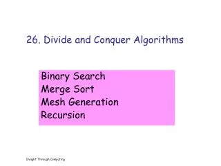
Divide-and-conquer algorithms Before we solve the general case, let us look at some more complex examples: • Searching an ordered matrix • Integer multiplication (Karatsuba algorithm) • Matrix multiplication
Searching an ordered matrix Consider an n×n matrix where each row and column is linearly ordered; for example: • How can we determine if 19 is in the matrix?
Searching an ordered matrix Consider the following search for 19: • Search across until ai,j + 1 > 19 • Alternate between • Searching down until ai,j > 19 • Searching back until ai,j < 19 This requires us to check at most 3n entries: O(n)
Searching an ordered matrix Can we do better than O(n)? Logically, no: any number could appear in up to n positions, each of which must be checked • Never-the-less: let’s generalize checking the middle entry
Searching an ordered matrix 17 < 19, and therefore, we can only exclude the top-left sub-matrix:
Searching an ordered matrix Thus, we must recursively search three of the four sub-matrices • Each sub-matrix is approximately n/2 × n/2
Searching an ordered matrix If the number we are searching for was less than the middle element, e.g., 9, we would have to search three different squares
Searching an ordered matrix Thus, the recurrence relation must be because • T(n) is the time to search a matrix of size n × n • The matrix is divided into 4 sub-matrices of size n/2 × n/2 • Search 3 of those sub-matrices • At each step, we only need compare the middle element: Q(1)
Searching an ordered matrix We can solve the recurrence relationship using Maple: > rsolve( {T(n) = 3*T(n/2) + 1, T(1) = 1}, T(n) ); > evalf( log[2]( 3 ) );
Searching an ordered matrix Therefore, this search is approximately O(n1.585), which is significantly worse than a linear search:
Searching an ordered matrix Note that it is T(n) = 3T(n/2) + Q(1) and not T(n) = 3T(n/4) + Q(1) We are breaking the n × nmatrix into four (n/2) × (n/2) matrices If N = n2, then we could write T(N) = 3T(N/4) + Q(1)
Searching an ordered matrix Where is such a search necessary? Consider a bi-parental heap Without proof, most operations are O( ) including searches Binary heaps: most operations are O(ln(n)) but searches are O(n)
Searching an ordered matrix For example, consider a search for the value 44: The matrix has n entries in See: http://ece.uwaterloo.ca/~dwharder/aads/Algorithms/Beaps/
Searching an ordered matrix Note: the linear searching algorithm is only optimal for square matrices • A binary search would be optimal for a 1 ×n or n× 1 matrix • Craig Gidney posts an interesting discussion on such searches when the matrix is not close to square http://twistedoakstudios.com/blog/Post5365_searching-a-sorted-matrix-faster
Integer multiplication Calculate the product of two 16-digit integers 3563474256143563 × 8976558458718976 Multiplying two n-digit numbers requires Q(n2) multiplications of two decimal digits: 3563474256143563 × 8976558458718976 21380845536861378 24944319793004941 32071268305292067 28507794049148504 3563474256143563 24944319793004941 28507794049148504 17817371280717815 14253897024574252 28507794049148504 17817371280717815 17817371280717815 21380845536861378 24944319793004941 32071268305292067 + 28507794049148504 . 31987734976412811376690928351488 n
Integer multiplication Rewrite the product 3563474256143563 × 8976558458718976 as (35634742 × 108 + 56143563) × (89765584×108 + 58718976) which requires four multiplications of 8-digit integers: (35634742 ×89765584)×1016 + (35634742 ×58718976+ 56143563 ×89765584)×108 + (56143563 ×58718976) Adding two n-digit integers is a Q(n) operation
Integer multiplication Thus, the recurrence relation is: Again, we solve the recurrence relation using Maple: > rsolve( {T(n) = 4*T(n/2) + n, T(1) = 1}, T(n) ); This is still Q(n2)
Integer multiplication To reduce the run time, the Karatsuba algorithm (1961) reduces the number of multiplications Let x = 3563474256143563 y = 8976558458718976 and define xMS = 35634742 xLS= 56143563 yMS = 89765584 yLS = 58718976 and thus x = xMS×108 + xLS y = yMS×108 + yLS
Integer multiplication The multiplication is now: xy = xMSyMS×1016 + (xLyR + xRyL)×108 + xLSyLS Rewrite the middle product as xMSyLS + xLSyMS = (xLS– xMS)(yLS– yMS) + xMSyMS + xLSyLS Two of these are already calculated!
Integer multiplication Thus, the revised recurrence relation may again be solved using Maple: > rsolve( {T(n) = 3*T(n/2) + n, T(1) = 1}, T(n) ); where log2(3) ≈ 1.585
Integer multiplication Plotting the two functions n2 and n1.585, we see that they are significantly different
Integer multiplication This is the same asymptotic behaviour we saw for our alternate searching behaviour of an ordered matrix, however, in this case, it is an improvement on the original run time! Even more interesting is that the recurrence relation are different: • T(n) = 3T(n/2) + Q(n) integer multiplication • T(n) = 3T(n/2) + Q(1) searching an ordered matrix
Integer multiplication In reality, you would probably not use this technique: there are others There are also libraries available for fast integer multiplication For example, the GNU Image Manipulation Program (GIMP) comes with a complete set of tools for fast integer arithmetic http://www.gimp.org/
Integer multiplication The Toom-Cook algorithm (1963 and 1966) splits the integers into k parts and reduces the k2 multiplicationsto 2k – 1 • Complexity is Q(nlogk(2k – 1)) • Karatsuba is a special case when k = 2 • Toom-3 (k = 3) results in a run time of Q(nlog3(5)) = Q(n1.465) The Schönhage-Strassen algorithm runs inQ(n ln(n) ln(ln(n))) time but is only useful for very large integers (greater than 10 000 decimal digits)
Matrix multiplication Consider multiplying two n ×n matrices, C = AB This requires the Q(n) dot product of each of the n rows of A with each of the n columns of B The run time must be Q(n3) • Can we do better? j ci,j i
Matrix multiplication In special cases, faster algorithms exist: • If both matrices are diagonal or tri-diagonal Q(n) • If one matrix is diagonal or tri-diagonal Q(n2) In general, however, this was not believed to be possible to do better
Matrix multiplication Consider this product of two n ×n matrices • How can we break this down into smaller sub-problems?
Matrix multiplication Break each matrix into four (n/2) × (n/2) sub-matrices • Write each sub-matrix of C as a sum-of-products A B C
Matrix multiplication Justification: cij is the dot product of the ith row of A and the jth column of B ci,j
Matrix multiplication This is equivalent for each of the sub-matrices:
Matrix multiplication We must calculate the four sums-of-products C00 = A00B00 + A01B10 C01 = A00B01 + A01B11 C10 = A10B00 + A11B10 C11 = A10B01 + A11B11 This totals 8 products of (n/2) × (n/2) matrices • This requires four matrix-matrix additions: Q(n2)
Matrix multiplication The recurrence relation is: Using Maple: > rsolve( {T(n) = 8*T(n/2) + n^2, T(1) = 1}, T(n) );
Matrix multiplication In 1969, Strassen developed a technique for performing matrix-matrix multiplication in Q(nlg(7)) ≈ Q(n2.807) time • Reduce the number of matrix-matrix products
Matrix multiplication Consider the following seven matrix products M1 = (A00 – A10)(B00 + B01) M2 = (A00 + A11)(B00 + B11) M3 = (A01 – A11)(B10 + B11) M4 = A00(B01 – B11) M5 = A11(B10 – B00) M6 = (A10 + A11)B00 M7 = (A00 + A01)B11 • The four sub-matrices of C may be written as • C00 = M3 + M2 + M5 – M7 • C01 = M4 + M7 • C10 = M5 + M6 • C11 = M2 – M1 + M4 – M6
Matrix multiplication Thus, the new recurrence relation is: Using Maple: > rsolve( {T(n) = 7*T(n/2) + n^2, T(1) = 1}, T(n) );
Matrix multiplication Note, however, that there is a lot of additional work required Counting additions and multiplications: Classic2n3 – n2 Strassen7nlg(7) – 6 n2
Matrix multiplication Examining this plot, and then solving explicitly, we find that Strassen’s method only reduces the number of operations for n > 654 • Better asymptotic behaviour does not immediately translate into better run-times The Strassen algorithm is not the fastest • the Coppersmith–Winograd algorithm runs in Q(n2.376) time but the coefficients are too large for any problem Therefore, better asymptotic behaviour does not immediately translate into better run-times
Observation Some literature lists the run-time as O(7lg(n)) Recall that these are equal: 7lg(n) = nlg(7) Proof: 7lg(n) = (2lg(7)) lg(n) = 2lg(7) lg(n) = 2lg(n) lg(7) = (2lg(n)) lg(7) = n lg(7)
Fast Fourier transform The last example is the fast Fourier transform • This takes a vector from the time domain to the frequency domain The Fourier transform is a linear transform • For finite dimensional vectors, it is a matrix-vector product Fnx http://xkcd.com/26/
Fast Fourier transform To perform a linear transformation, it is necessary to calculate a matrix-vector product:
Fast Fourier transform We can apply a divide and conquer algorithm to this problem • Break the matrix-vector product into four matrix-vector products, each of half the size