Download
1 / 10
150 likes | 371 Views
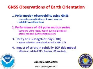
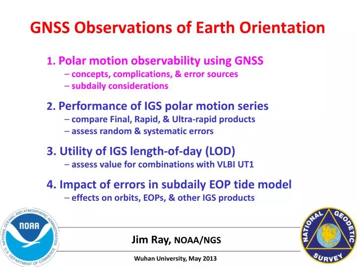
1. Polar motion observability using GNSS concepts, complications, & error sources subdaily considerations 2. Performance of IGS polar motion series compare Final, Rapid, & Ultra-rapid products assess random & systematic errors 3. Utility of IGS length -of- day (LOD)

E N D
1. Polar motion observability using GNSS • concepts, complications, & error sources • subdaily considerations • 2. Performance of IGS polar motion series • compare Final, Rapid, & Ultra-rapid products • assess random & systematic errors • 3. Utility of IGS length-of-day (LOD) • assess value for combinations with VLBI UT1 • 4. Impact of errors in subdaily EOP tide model • effects on orbits, EOPs, & other IGS products GNSS Observations of Earth Orientation Jim Ray, NOAA/NGS Wuhan University, May 2013
Earth Orientation Parameters (EOPs) • EOPs are the five angles used to relate points in the Terrestrial & Celestial Reference Frames: [CRF] = P · N(ψ, ε) · R(UT1) · W(xp , yp) · [TRF] • Precession-Nutation describes the motion of the Earth’s rotation axis in inertial space • Rotation about axis given by UT1 angle • Wobble of pole in TRF given by terrestrial coordinates of polar motion (xp , yp) • But only three angles, not five, are independent • this conventional form is used to distinguish excitation sources: • Nutation ↔ driven by gravitational potentials outside Earth system • Polar Motion ↔ driven by internal redistributions of mass/momentum • separation of Nutation & Polar Motion estimates given by convention (xp, yp) 02
Separation of Nutation & Polar Motion • Motions defined in frequency domain • note that diurnal retrograde motion in TRF is fixed in CRF: -1.0 cycle per sidereal day (TRF) = 0.0 cycles per sidereal day (CRF) • Because GNSS cannot observe CRF (quasar frame), it does not measure precession-nutation or UT1 • but GNSS can sense nutation-rate & UT1-rate (LOD) changes • GNSS is superb for Polar Motion due to robust global tracking network • pole position is essentially an unmarked point in the TRF frequency in Terrestrial Frame ← polar motion polar motion → frequency in Celestial Frame precession nutation 03
Observability of Polar Motion (PM) • Suppose a priori pole position has some unknown error: • Due to diurnal Earth spin, PM error causes sinusoidal apparent motion for all TRF points as viewed from GNSS satellite frame • (xp, yp) partials are simple diurnal sine waves • amplitude & phase depend only on station XYZ location • quality of PM estimates depends mostly on Earth coverage by GNSS stations • IGS formal errors: σx,y = 5 µas actual pole position assumed pole position Signature of PM error in GNSS Observations ←1 solar day → 04
Some Observability Complications • GPS satellites have period of ~0.5 sidereal day • ground tracks repeat every ~1 sidereal day • differs from 1 solar day by only ~4 minutes • other GNSS constellations have longer or shorter periods • any common-mode near-diurnal orbit errors can alias into PM estimates • Any other net diurnal sinusoidal error in GNSS orbits will also alias into PM estimates • main error comes from model for 12h/24h EOP tides • mostly caused by EOP effect of ocean tidal motions • current IERS model has errors at < ~20% • Other common mode effects could also be important: • diurnal temperature effects (e.g., heights of GNSS stations) • diurnal troposphere modeling errors • various other tidal modeling errors • local station multipath signatures due to ground repeat period 05
On “Subdaily" Polar Motion ← subdaily retrograde PM subdailyprograde PM → frequency in Terrestrial Frame • First, “subdaily” polar motion is not a well-defined concept • overlaps with nutation band in retrograde sense • inseparable from a global rotation of satellite frame • so constraint normally applied to block diurnal retrograde frequencies • this is effectively a filter with poor response for GNSS arcs of ~1 day [D. Thaller et al., J. Geodesy, 2007] • Second, observability is reduced for intervals <1 solar day • partial diurnal sinusoidal cannot be separated from other parameters • so parameter continuity is required for direct subdaily estimates • most common approach (Bern group) is to use 1 hr continuous segments • this operates as another filter, but with other disadvantages (next slides) • So subdaily results are easily affected by spurious effects ← polar motion precession nutation polar motion → 06
Effects of “Continuity Filter” (1/3) • Compare offset + rate to continuous linear segments (CLS) • IGS requests daily PM estimates as mid-day offsets + rates • but some Analysis Centers prefer CLS approach • results are not equivalent near Nyquist frequency • CLS results are non-physical at high freqs • Consider cosine wave at Nyquistfreq • φ = π • CLS & offset + rate give exactly same estimates for this phase • Now shift cosine by -90° • φ = π/2 • CLS estimates are all 0.0 • but offset + rate estimates are not zero & not constant CLS estimation Offset + rate estimation 07
Effects of “Continuity Filter” (2/3) • CLS attenuates Nyquist signal amplitudes by factor of 2 • power reduced by factor of 4 at Nyquist frequency • power starts dropping at ~0.6 x Nyquist frequency & higher • Filter effect clearly seen in IGS PM results • most Analysis Centers follow f-4 power law for sub-seasonal periods, e.g., GFZ (below right, during 11 Mar 2005 – 29 Dec 2007) • but CODE used CLS parameters & had strong high-freq smoothing Smoothed PSD for Reprocessed CODE PM Smoothed PSD for Reprocessed GFZ PM 08
Effects of “Continuity Filter” (3/3) • CLS method is not a simple smoothing filter • it distorts signal content by attenuating certain phases over others • causes all parameters to be strongly correlated at all times • should not be used when signals of interest are near Nyquist sampling • Unfiltered IGS daily PM can be extrapolated to estimate subdaily PM variance (non-tidal) • sub-seasonal PSD follows f-4 power law (integrated random walk process) • fits to GFZ PSD over 0.1 to 0.5 cpd: PSDx(f) = (48.11 µas2/cpd) * (f/cpd)-4.55 PSDy(f) = (64.21 µas2/cpd) * (f/cpd)-4.10 • if valid at f > 0.5 cpd, then integrate over 1 cpd → infinity: σ2x(subdaily) = 13.55 µas2 σ2y(subdaily) = 20.73 µas2 • much too small to be detectable Smoothed PSD for Reprocessed GFZ PM 09
Estimating “Subdaily" PM • Three methods probably feasible: • Kalman filter • use normal deterministic PM parameters for daily offset + rate • add stochastic model (f-4 integrated random walk) to estimate deviations • probably can be done with JPL’s GIPSY, but I know of no results • CLS • only method used till now • but problems noted above are serious & probably gives unreliable results • invert from overlapping daily fits • in principle, probably could invert normal daily offset + rate fits • but use overlapping data arcs (highly correlated estimates) • would probably need to add f-4 integrated random walk model to inversion • not known to be tried • could be tested using IGS Ultra-rapid PM series (24 hr arcs with 6 hr time steps) • Subdaily PM (non-tidal) power is so small, no clear reason to try to measure • but filling band from 0.5 to 1.0 cpd could aid excitation studies (e.g., using IGS Ultras) 10