Download

1 / 55
900 likes | 1.83k Views
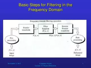
Frequency Domain Filtering (Chapter 4). CS474/674 - Prof. Bebis. Frequency Domain Methods. Frequency Domain. Spatial Domain. Major filter categories. Typically, filters are classified by examining their properties in the frequency domain: (1) Low-pass (2) High-pass (3) Band-pass

E N D
Frequency Domain Filtering (Chapter 4) CS474/674 - Prof. Bebis
Frequency Domain Methods Frequency Domain Spatial Domain
Major filter categories • Typically, filters are classified by examining their properties in the frequency domain: (1) Low-pass (2) High-pass (3) Band-pass (4) Band-stop
Example Original signal Low-pass filtered High-pass filtered Band-pass filtered Band-stop filtered
frequency domain time domain Low-pass filters(i.e., smoothing filters) • Preserve low frequencies - useful for noise suppression
time domain frequency domain High-pass filters(i.e., sharpening filters) • Preserves high frequencies - useful for edge detection
frequency domain time domain Band-pass filters • Preserves frequencies within a certain band
Band-stop filters • How do they look like? Band-stop Band-pass
Frequency Domain Methods Case 1: h(x,y) is given in the spatial domain. Case 2: H(u,v) is given in the frequency domain.
Frequency domain filtering: steps F(u,v) = R(u,v) + jI(u,v)
Frequency domain filtering: steps (cont’d) G(u,v)= F(u,v)H(u,v) = H(u,v) R(u,v) + jH(u,v)I(u,v)
Example fp(x,y) f(x,y) fp(x,y)(-1)x+y F(u,v) G(u,v)=F(u,v)H(u,v) H(u,v) - centered g(x,y) gp(x,y)
h(x,y) specified in spatial domain:How to generate H(u,v) from h(x,y)? • If h(x,y) is given in the spatial domain, we can generate H(u,v) as follows: • Form hp(x,y) by padding with zeroes. 2. Multiply by (-1)x+y to center its spectrum. 3. Compute its DFT to obtain H(u,v)
Example: h(x,y) is specified in the spatial domain 600 x 600 Important: need to preserve odd symmetry (i.e., H(u,v) should be imaginary) (read details on page 268) Sobel
Results of Filtering in the Spatial and Frequency Domains spatial domain filtering frequency domain filtering
Example • Consider a filter H(u,v) that is 0 at the center of the transform and 1 elsewhere • What can you say for the output image? zero average intensity
Low-pass (LP) filtering • Preserves low frequencies, attenuates high frequencies. ideal in practice D0: cut-off frequency
Lowpass (LP) filtering (cont’d) • In 2D, the cutoff frequencies lie on a circle.
Specifying a 2D low-pass filter • Specify cutoff frequencies by specifying the radius of a circle centered at point (N/2, N/2) in the frequency domain. • The radius is chosen by specifying the percentage of total power enclosed by the circle.
Specifying a 2D low-pass filter (cont’d) • Typically, most frequencies are concentrated around the center of the spectrum. r=8 (90% power) r=18 (93% power) original r: radius r=43 (95%) r=78 (99%) r=152 (99.5%)
How does D0 control smoothing? • Reminder: multiplication in the frequency domain implies convolution in the time domain time domain freq. domain * =
How does D0 control smoothing? (cont’d) • D0 controls the amount of blurring r=78 (99%) r=8 (90%)
Ringing Effect • Sharp cutoff frequencies produce an overshoot of image features whose frequency is close to the cutoff frequencies (ringing effect). h=f*g
Low Pass (LP) Filters • Ideal low-pass filter (ILPF) • Butterworth low-pass filter (BLPF) • Gaussian low-pass filter (GLPF)
Butterworth LP filter (BLPF) • In practice, we use filters that attenuate high frequencies smoothly (e.g., Butterworth LP filter) less ringing effect n=1 n=4 n=16
Spatial Representation of BLPFs n=1 n=2 n=5 n=20
Comparison: Ideal LP and BLPF BLPF ILPF D0=10, 30, 60, 160, 460 D0=10, 30, 60, 160, 460 n=2
Gaussian: Frequency – Spatial Domains spatial domain frequency domain
Examples of smoothing by GLPF (2) D0=100 D0=80
High-Pass filtering • A high-pass filter can be obtained from a low-pass filter using: = 1 - D0
High-pass filtering (cont’d) • Preserves high frequencies, attenuates low frequencies.
High Pass (LP) Filters • Ideal high-pass filter (IHPF) • Butterworth high-pass filter (BHPF) • Gaussian high-pass filter (GHPF) • Difference of Gaussians • Unsharp Masking and High Boost filtering
Butterworth high pass filter (BHPF) • In practice, we use filters that attenuate low frequencies smoothly (e.g., Butterworth HP filter) less ringing effect
Spatial Representation of High-pass Filters IHPF BHPF GHPF
Comparison: IHPF and BHPF IHPF D0=30,60,160 D0=30,60,160 n=2 BHPF
Gaussian HP filter GHPF BHPF
Comparison: BHPF and GHPF D0=30,60,160 BHPF n=2 D0=30,60,160 GHPF
Example: High-pass Filtering and Thresholding for Fingerprint Image Enhancement BHPF (order 4 with a cutoff frequency 50)
Difference of Gaussians:Frequency – Spatial Domains This is a high-pass filter!
Difference of Gaussians:Frequency – Spatial Domains (cont’d) spatial domain frequency domain High-pass filter!
Frequency Domain Analysis of Unsharp Masking and Highboost Filtering Unsharp Masking: Highboost filtering: (alternative definition) previous definition: Frequency domain:
Revisit: Unsharp Masking and Highboost Filtering Highboost Filter
Highboost and High-Frequency-Emphasis Filters 1+k k1+k2 1 k1 Highboost High-emphasis
Example GHPF D0=40 High-emphasis High-emphasis and hist. equal. High-Frequency Emphasis filtering Using Gaussian filter k1=0.5, k2=0.75
Homomorphic filtering • Many times, we want to remove shading effects from an image (i.e., due to uneven illumination) • Enhance high frequencies • Attenuate low frequencies but preserve fine detail.
Homomorphic Filtering (cont’d) • Consider the following model of image formation: • In general, the illumination component i(x,y) varies slowly and affects low frequencies mostly. • In general, the reflection component r(x,y) varies faster and affects high frequencies mostly. i(x,y): illumination r(x,y): reflection IDEA: separate low frequencies due to i(x,y) from high frequencies due to r(x,y)
How are frequencies mixed together? • Low and high frequencies from i(x,y) and r(x,y) are mixed together. • When applying filtering, it is difficult to handle low/high frequencies separately.
Can we separate them? • Idea: Take the ln( ) of