Download
1 / 106
1.06k likes | 1.07k Views
This paper explores Proper Orthogonal Decomposition (POD) closure models for stable POD-Galerkin Reduced Order Models (ROMs) in fluid problems, with a focus on long-time integration and extreme model reduction. The methods presented in the paper are alternatives to existing work on basis rotation for stabilization and enhancement of projection-based ROMs for the compressible Navier-Stokes equations.

E N D
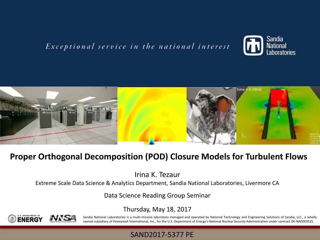
Proper Orthogonal Decomposition (POD) Closure Models for Turbulent Flows Irina K. Tezaur Extreme Scale Data Science & Analytics Department, Sandia National Laboratories, Livermore CA Data Science Reading Group Seminar Thursday, May 18, 2017 Sandia National Laboratories is a multi-mission laboratory managed and operated by National Technology and Engineering Solutions of Sandia, LLC., a wholly owned subsidiary of Honeywell International, Inc., for the U.S. Department of Energy’s National Nuclear Security Administration under contract DE-NA0003525. SAND2017-5377 PE
Paper • My interest in this work:
Paper • My interest in this work: • I am interested in stable POD-GalerkinROMs for fluid problems (next slides).
Paper • My interest in this work: • I am interested in stable POD-GalerkinROMs for fluid problems (next slides). • Authors of this paper have similar requirements for ROMs as me: use ROMs for long-time integration, “extreme model reduction”, QoI = statistics of flow, etc.
Paper • My interest in this work: • I am interested in stable POD-GalerkinROMs for fluid problems (next slides). • Authors of this paper have similar requirements for ROMs as me: use ROMs for long-time integration, “extreme model reduction”, QoI = statistics of flow, etc. • Methods in this paper are alternatives to my work on basis rotation1. 1 M. Balajewicz, I. Tezaur, E. Dowell. "Minimal subspace rotation on the Stiefel manifold for stabilization and enhancement of projection-based reduced order models for the compressible Navier-Stokes equations", JCP321 (2016) 224-241.
Paper • My interest in this work: • I am interested in stable POD-GalerkinROMs for fluid problems (next slides). • Authors of this paper have similar requirements for ROMs as me: use ROMs for long-time integration, “extreme model reduction”, QoI = statistics of flow, etc. • Methods in this paper are alternatives to my work on basis rotation1. • I am working with T. Iliescu to try to understand how to extend methods such as those in the paper to compressible flow problems and to make them more rigorous. 1 M. Balajewicz, I. Tezaur, E. Dowell. "Minimal subspace rotation on the Stiefel manifold for stabilization and enhancement of projection-based reduced order models for the compressible Navier-Stokes equations", JCP321 (2016) 224-241.
Outline • Motivation/Background • Section 2: POD/Galerkin ROMs for Incompressible Flows • Background on Turbulence Modeling/Large Eddy Simulation • 4. Section 3: POD Closure Models • Mixing Length (ML) • Smagorinsky (S) • Variational Multi-Scale (VMS) • Dynamic Subgrid (DS) • Section 4.1: Computational Efficiency • 6. Section 4.2: Numerical Results for 3D Flow Around Cylinder • 7. Section 5 and Beyond: Future/Follow-Up Work • [8. Basis Rotation (My Work – an Alternative Approach)]
Outline • Motivation/Background • Section 2: POD/Galerkin ROMs for Incompressible Flows • Background on Turbulence Modeling/Large Eddy Simulation • 4. Section 3: POD Closure Models • Mixing Length (ML) • Smagorinsky (S) • Variational Multi-Scale (VMS) • Dynamic Subgrid (DS) • Section 4.1: Computational Efficiency • 6. Section 4.2: Numerical Results for 3D Flow Around Cylinder • 7. Section 5 and Beyond: Future/Follow-Up Work • [8. Basis Rotation (My Work – an Alternative Approach)]
Motivation • We are interested in the compressible captive-carry problem.
Motivation • We are interested in the compressible captive-carry problem. • Of primary interest are long-time predictive simulations: ROM run at same parameters as FOM but much longer in time.
Motivation • We are interested in the compressible captive-carry problem. • Of primary interest are long-time predictive simulations: ROM run at same parameters as FOM but much longer in time. • QoIs: statistics of flow, e.g., pressure Power Spectral Densities (PSDs) [right].
Motivation • We are interested in the compressible captive-carry problem. • Of primary interest are long-time predictive simulations: ROM run at same parameters as FOM but much longer in time. • QoIs: statistics of flow, e.g., pressure Power Spectral Densities (PSDs) [right]. • Secondary interest: ROMs robust w.r.t. parameter changes (e.g., Reynolds, Mach number) for enabling uncertainty quantification.
Proper Orthogonal Decomposition (POD)/ Galerkin method to model reduction High fidelity CFD simulations: Snapshot 1 Snapshot 2 Snapshot K Fluid modal decomposition (POD): Galerkin projection of fluid PDEs: Step 1 Step 2 • Snapshot matrix: , …, • SVD: • Truncation:) Basis energy = FOM = full order model # of dofs in FOM # of snapshots # of dofs in ROM (, ) “Small” ROM ODE system: )
Extreme Model Reduction • Most realistic applications (e.g., high Re compressible cavity): basis that captures 99% snapshot energy is required to accurately reproduce snapshots. • leads to >except for toy problems and/or low-fidelity models. • Higher order modes are in general unreliable for prediction, so including them in the basis is unlikely to improve the predictive capabilities of a ROM. Figure (right) shows projection error for POD basis constructed using 800 snapshots for cavity problem. Dashed line = end of snapshot collection period. We are looking for an approach that enables extreme model reduction: ROM basis size is or .
Mode truncation instability Projection-based MOR necessitates truncation.
Mode truncation instability Projection-based MOR necessitates truncation. • POD is, by definition and design, biased towards the large, energy producingscales of the flow (i.e., modes with large POD eigenvalues).
Mode truncation instability Projection-based MOR necessitates truncation. • POD is, by definition and design, biased towards the large, energy producingscales of the flow (i.e., modes with large POD eigenvalues). • Truncated/unresolved modes are negligible from a data compressionpoint of view (i.e., small POD eigenvalues) but are crucial for the dynamical equations.
Mode truncation instability Projection-based MOR necessitates truncation. • POD is, by definition and design, biased towards the large, energy producingscales of the flow (i.e., modes with large POD eigenvalues). • Truncated/unresolved modes are negligible from a data compressionpoint of view (i.e., small POD eigenvalues) but are crucial for the dynamical equations. • For fluid flow applications, higher-order modes are associated with energy dissipation
Mode truncation instability Projection-based MOR necessitates truncation. • POD is, by definition and design, biased towards the large, energy producingscales of the flow (i.e., modes with large POD eigenvalues). • Truncated/unresolved modes are negligible from a data compressionpoint of view (i.e., small POD eigenvalues) but are crucial for the dynamical equations. • For fluid flow applications, higher-order modes are associated with energy dissipation low-dimensional ROMs can be inaccurate and unstable.
Mode truncation instability Projection-based MOR necessitates truncation. • POD is, by definition and design, biased towards the large, energy producingscales of the flow (i.e., modes with large POD eigenvalues). • Truncated/unresolved modes are negligible from a data compressionpoint of view (i.e., small POD eigenvalues) but are crucial for the dynamical equations. • For fluid flow applications, higher-order modes are associated with energy dissipation low-dimensional ROMs can be inaccurate and unstable. For a low-dimensional ROM to be stable and accurate, the truncated/unresolved subspacemust be accounted for.
Mode truncation instability Projection-based MOR necessitates truncation. • POD is, by definition and design, biased towards the large, energy producingscales of the flow (i.e., modes with large POD eigenvalues). • Truncated/unresolved modes are negligible from a data compressionpoint of view (i.e., small POD eigenvalues) but are crucial for the dynamical equations. • For fluid flow applications, higher-order modes are associated with energy dissipation low-dimensional ROMs can be inaccurate and unstable. For a low-dimensional ROM to be stable and accurate, the truncated/unresolved subspacemust be accounted for. Turbulence Modeling (this paper) Subspace Rotation (our approach)
Outline • Motivation/Background • Section 2: POD/Galerkin ROMs for Incompressible Flows • Background on Turbulence Modeling/Large Eddy Simulation • 4. Section 3: POD Closure Models • Mixing Length (ML) • Smagorinsky (S) • Variational Multi-Scale (VMS) • Dynamic Subgrid (DS) • Section 4.1: Computational Efficiency • 6. Section 4.2: Numerical Results for 3D Flow Around Cylinder • 7. Section 5 and Beyond: Future/Follow-Up Work • [8. Basis Rotation (My Work – an Alternative Approach)]
Section 2: POD-Galerkin-ROM (POD-G-ROM) for Incompressible Flow • Governing equations of incompressible flow:
Section 2: POD-Galerkin-ROM (POD-G-ROM) for Incompressible Flow • Governing equations of incompressible flow: • POD approximation of velocity solution2: where = base flow, = POD modes. 2 Pressure ROM can be obtained by solving pressure-Poisson equation. Pressure term drops out from (1) following projection due to BCs. See [36,56].
Section 2: POD-Galerkin-ROM (POD-G-ROM) for Incompressible Flow • Governing equations of incompressible flow: • POD approximation of velocity solution2: • where = base flow, = POD modes. • Projecting (1) onto reduced basis , the following POD-G(alerkin)-ROM is obtained: where = reduced subspace, = deformation tensor of . 2 Pressure ROM can be obtained by solving pressure-Poisson equation. Pressure term drops out from (1) following projection due to BCs. See [36,56].
Section 2: POD-G-ROM for Incompressible Flow • POD-G-ROM algebraic system: where:
Section 2: POD-G-ROM for Incompressible Flow • POD-G-ROM algebraic system: where: • POD-G-ROM in matrix form: (8)
Section 2: POD-G-ROM for Incompressible Flow • POD-G-ROM algebraic system: where: • POD-G-ROM in matrix form: (8) • POD-G-ROM (8) has been successfully used for laminar flows.
Section 2: POD-G-ROM for Incompressible Flow • POD-G-ROM algebraic system: where: • POD-G-ROM in matrix form: (8) • POD-G-ROM (8) has been successfully used for laminar flows. • For structurally-dominated turbulent flows, POD-G-ROM fails: effect of discarded modes need to be included in some way.
Section 2: POD-G-ROM for Incompressible Flow • POD-G-ROM algebraic system: where: • POD-G-ROM in matrix form: (8) • POD-G-ROM (8) has been successfully used for laminar flows. • For structurally-dominated turbulent flows, POD-G-ROM fails: effect of discarded modes need to be included in some way. “POD closure problem”
Outline • Motivation/Background • Section 2: POD/Galerkin ROMs for Incompressible Flows • Background on Turbulence Modeling/Large Eddy Simulation • 4. Section 3: POD Closure Models • Mixing Length (ML) • Smagorinsky (S) • Variational Multi-Scale (VMS) • Dynamic Subgrid (DS) • Section 4.1: Computational Efficiency • 6. Section 4.2: Numerical Results for 3D Flow Around Cylinder • 7. Section 5 and Beyond: Future/Follow-Up Work • [8. Basis Rotation (My Work – an Alternative Approach)]
Turbulence • For sufficiently high Reynolds number, flow becomes turbulent.
Turbulence • For sufficiently high Reynolds number, flow becomes turbulent. • Turbulence is nonlinear, chaotic, 3D phenomenon.
Turbulence • For sufficiently high Reynolds number, flow becomes turbulent. • Turbulence is nonlinear, chaotic, 3D phenomenon. • Kolmogorov hypothesis / energy cascade: • Kinetic energy enters the turbulence through the production mechanism at largest scales of motion. • Energy is transferred (by inviscid processes) to smaller and smaller scales. • At smallest scales, energy is dissipated by viscous action.
Turbulence Modeling • Direct Numerical Simulation (DNS): solves full Navier-Stokes (NS) equations (1) requires fine meshes in boundary layer to resolve fine scales. • Too computationally expensive to be feasible for realistic complex flows. • Large Eddy Simulation (LES): reduces computational cost of DNS by ignoring smallest length scales (most computationally expensive to resolve). • LES equations obtained by low-pass-filtering full NS equations. • Reynolds Averaged Navier-Stokes (RANS): time-averaged versions of NS equations turbulence is modeled, not resolved.
Large Eddy Simulation (LES) E(k) = energy spectrum Left: energy cascade / “Kolmogorov spectrum” (energy transfer from large to small scales); LES filter filters out small scales. • Four conceptual steps of LES (Pope, Chapter 13): • (i) Filtering operation to decompose velocity into filtered (or resolved) component ssss and residual (or subgrid-scale) component • (ii) Equations for evolution of the filtered velocity are derived from the NS equations. • (iii) Closure is obtained by modeling the residual-stress tensor (most simply with eddy- viscosity model). • (iv) Model filtered equations are solved numerically for , which provides approximation of large-scale motions in one realization of turbulent flow.
LES Filtering • General filtering operation defined by: where is a specified rapidly-decaying “filter function”, which has an associated “cut-off” length and time scale. Scales smaller than these cut-offs are eliminated using filter.
LES Filtering • General filtering operation defined by: where is a specified rapidly-decaying “filter function”, which has an associated “cut-off” length and time scale. Scales smaller than these cut-offs are eliminated using filter. Bold: filtered signal • Given a filter, any field can be split up into filtered and sub-filtered scale:
LES Filtered Governing Equations • Applying filtering operation to (1) gives the following equations for the filtered variables: ( where is the subfilter-scale stress tensor:
LES Filtered Governing Equations • Applying filtering operation to (1) gives the following equations for the filtered variables: ( where is the subfilter-scale stress tensor: • is most difficult term to model, as it requires knowledge of unfiltered velocity field, which is unknown.
LES Filtered Governing Equations • Applying filtering operation to (1) gives the following equations for the filtered variables: ( where is the subfilter-scale stress tensor: • is most difficult term to model, as it requires knowledge of unfiltered velocity field, which is unknown. • Common approaches to model : eddy-viscosity (EV) models • where is the eddy-viscosity. • Expression for : “eddy-viscosity ansatz” • Examples: mixing-length, Smagorinsky, etc. – parameters based on Kolmogorov spectrum.
Outline • Motivation/Background • Section 2: POD/Galerkin ROMs for Incompressible Flows • Background on Turbulence Modeling/Large Eddy Simulation • 4. Section 3: POD Closure Models • Mixing Length (ML) • Smagorinsky (S) • Variational Multi-Scale (VMS) • Dynamic Subgrid (DS) • Section 4.1: Computational Efficiency • 6. Section 4.2: Numerical Results for 3D Flow Around Cylinder • 7. Section 5 and Beyond: Future/Follow-Up Work • [8. Basis Rotation (My Work – an Alternative Approach)]
Section 3.3: POD Closure Models • POD-G-ROM(8) has been successfully used for laminar flows. • For structurally-dominated turbulent flows, POD-G-ROM fails: effect of discarded modes need to be included in some way. “POD closure problem”
Section 3.3: POD Closure Models • POD-G-ROM(8) has been successfully used for laminar flows. • For structurally-dominated turbulent flows, POD-G-ROM fails: effect of discarded modes need to be included in some way. • Natural way to tackle POD closure problem: “eddy-viscosity” (EV) turbulence modeling. • EV model states that role of discarded modes is to extract energy from system. • Concept of energy cascade has been confirmed numerically in POD setting. “POD closure problem”
Section 3.3: POD Closure Models • POD-G-ROM(8) has been successfully used for laminar flows. • For structurally-dominated turbulent flows, POD-G-ROM fails: effect of discarded modes need to be included in some way. • Natural way to tackle POD closure problem: “eddy-viscosity” (EV) turbulence modeling. • EV model states that role of discarded modes is to extract energy from system. • Concept of energy cascade has been confirmed numerically in POD setting. • EV-POD-ROM formulation: “POD closure problem” (24) where and correspond to numerical discretization of EV closure model.
Section 3.3: POD Closure Models • POD-G-ROM(8) has been successfully used for laminar flows. • For structurally-dominated turbulent flows, POD-G-ROM fails: effect of discarded modes need to be included in some way. • Natural way to tackle POD closure problem: “eddy-viscosity” (EV) turbulence modeling. • EV model states that role of discarded modes is to extract energy from system. • Concept of energy cascade has been confirmed numerically in POD setting. • EV-POD-ROM formulation: “POD closure problem” (24) where and correspond to numerical discretization of EV closure model. (24) is equivalent to adding to equations (1) and projecting.
Section 3.3: POD Closure Models • POD-G-ROM(8) has been successfully used for laminar flows. • For structurally-dominated turbulent flows, POD-G-ROM fails: effect of discarded modes need to be included in some way. • Natural way to tackle POD closure problem: “eddy-viscosity” (EV) turbulence modeling. • EV model states that role of discarded modes is to extract energy from system. • Concept of energy cascade has been confirmed numerically in POD setting. • EV-POD-ROM formulation: “POD closure problem” (24) where and correspond to numerical discretization of EV closure model. (24) is equivalent to adding to equations (1) and projecting. • Four EV-POD-ROMsof the form (24) proposed/evaluated: • 1. ML-POD-ROM (ML = mixing length). 3. VMS-POD-ROM (VMS = variational multi-scale) • 2. S-POD-ROM (S = Smagorinsky). 4. DS-POD-ROM (DS = dynamic subgrid)
POD Filter and Lengthscale (Section 3.1-3.2) • POD/Galerkin projection filter (Section 3.1): • In POD, there is no explicit spatial filter used to develop LES-type POD closure models, a POD filter needs to be introduced. • Natural filter is Galerkin projection: for all , the Galerkin projection is the solution to the following equation: By doing POD/Galerkin projection to build the ROM, one is applying a filter. In the context of LES, filtered equations require introduction of closure model to model effect of neglected POD modes. This is where idea of adding EV models to ROM equations comes from.
POD Filter and Lengthscale (Section 3.1-3.2) • POD/Galerkin projection filter (Section 3.1): • In POD, there is no explicit spatial filter used to develop LES-type POD closure models, a POD filter needs to be introduced. • Natural filter is Galerkin projection: for all , the Galerkin projection is the solution to the following equation: By doing POD/Galerkin projection to build the ROM, one is applying a filter. In the context of LES, filtered equations require introduction of closure model to model effect of neglected POD modes. This is where idea of adding EV models to ROM equations comes from. • POD lengthscale(Section 3.2): implicitly defined by neglected modes where spatial average in homogeneous direction, are streamwise and spanwise dimensions of computational domain.