Download
1 / 11
120 likes | 246 Views
Time-Cost Evaluation. Actual (Actual Cost of Work Completed). Earned Value (EV) (Budgeted Cost of Work Completed). Planned Value (PV) (Budgeted Cost of Work Scheduled). Cost. 0. Time. Schedule Variance SV = EV – PV Positive SV Means Early Negative SV means Late. Cost Variance

E N D
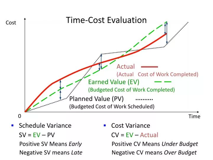
Time-Cost Evaluation Actual(Actual Cost of Work Completed) Earned Value (EV)(Budgeted Cost of Work Completed) Planned Value (PV)(Budgeted Cost of Work Scheduled) Cost 0 Time • Schedule Variance SV = EV – PV Positive SV Means Early Negative SV means Late • Cost Variance CV = EV – Actual Positive CV Means Under Budget Negative CV means Over Budget
Examples • Example 1 PV = $100, EV = $105, Actual = $95 • Example 2 PV = $100, EV = $80, Actual = $95 • Project is ______ worth of work __________ schedule • and ___________ budget. $5 ahead of $10 under • Project is ______ worth of work __________ schedule • and ___________ budget. $20 behind $15 over
Time-Cost Evaluation How much is the project ahead of schedule? $8000 – $7900 = $100 or $100 / $7900 = 1.3% early How much is the project above the budget? $8000 – $7500 = $500 or $500 / $8000 = 6.25% under budget
Sigma capability measures how many std.dev. the process mean is away from the closer tolerance limit Process Capability – Sigma Capability z1 z2 UTL LTL
Process Capability Index Suppose the control limits are X 3. If Cpk<1, then an “in-control” process might produce defects. • LTL = 70, UTL = 90, X = 80, = 2.5 Cpk = _______ • What if X shift to 84? Cpk = _______ 1.333 0.8
Improving Process Capability σ = 5 σ =10 LTL LTL UTL UTL σ =10 σ = 5 LTL LTL UTL UTL
Know The Enemy: 7 Types of Muda • Overproduction • Defects • Inventory (> need) • Waiting (of workers and products) • Processing (non adding value) • Motion (> minimum required) • Handling (> minimum required)
TPS Goal, Assumptions, Principles • Goal: Eliminate Waste (Muda) • TPS is a production system that is steeped in the philosophy of the complete elimination of all waste imbuing all aspects of production in pursuit of the most efficient methods. (www.toyota.co.jp/en/vision/production_system) • Assumptions: • Plan (in advance) <> Need (in real-time) • Problems will happen • Principles: • Just-In-Time (JIT) • Make problems visible, act immediately when they occur
Economic Order Quantity (EOQ) Model • Data: D = Demand rate (units / yr) C = Cost of purchasing or producing a unit ($ / unit) S = Setup cost or per order or per production run ($) H = Annual holding cost per unit of inventory ($ / (unit•yr)) H is often taken as a percentage of the unit cost: H = i C, where i is annual percentage holding cost • Decision: Q = Quantity of an order (units) • Objective: To minimize the total cost Let’s see how to compute the total cost …
Finding the Optimal Q (EOQ) Cost Lowest Cost Holding cost Ordering Cost QOPT (optimal order quantity) Q
Total Cost Inventory Slope = D (units/year) Number of orders per year = Annual ordering cost = Average inventory = Annual holding cost = Annual purchase cost = Q Time D / Q( / yr) (D / Q) S($ / yr) Q / 2(units) (Q / 2) H($ / yr) C D($ / yr)