Download
1 / 53
540 likes | 744 Views
Church, Kolmogorov and von Neumann: Their Legacy Lives in Complexity. Lance Fortnow NEC Laboratories America. 1903 – A Year to Remember. 1903 – A Year to Remember. 1903 – A Year to Remember. Kolmogorov. Church. von Neumann. Andrey Nikolaevich Kolmogorov.

E N D
Church, Kolmogorov and von Neumann:Their Legacy Lives in Complexity Lance Fortnow NEC Laboratories America
1903 – A Year to Remember Kolmogorov Church von Neumann
Andrey Nikolaevich Kolmogorov • Born:April 25, 1903Tambov, Russia • Died:Oct. 20, 1987
Alonzo Church • Born:June 14, 1903Washington, DC • Died:August 11, 1995
John von Neumann • Born:Dec. 28, 1903Budapest, Hungary • Died:Feb. 8, 1957
Frank Plumpton Ramsey • Born:Feb. 22, 1903Cambridge, England • Died:January 19, 1930 • Founder of Ramsey Theory
Applications of Ramsey Theory • Logic • Concrete Complexity • Complexity Classes • Parallelism • Algorithms • Computational Geometry
John von Neumann • Quantum • Logic • Game Theory • Ergodic Theory • Hydrodynamics • Cellular Automata • Computers
The Minimax Theorem (1928) • Every finite zero-sum two-person game has optimal mixed strategies. • Let A be the payoff matrix for a player.
The Yao Principle (Yao, 1977) • Worst case expected runtime of randomized algorithm for any input equals best case running time of a deterministic algorithm for worst distribution of inputs. • Invaluable for proving limitations of probabilistic algorithms.
Making a Biased Coin Unbiased • Given a coin with an unknown bias p, how do we get an unbiased coin flip?
Making a Biased Coin Unbiased • Given a coin with an unknown bias p, how do we get an unbiased coin flip? HEADS TAILS Flip Again or
Making a Biased Coin Unbiased • Given a coin with an unknown bias p, how do we get an unbiased coin flip? HEADS p(1-p) TAILS (1-p)p Flip Again or
Weak Random Sources • Von Neumann’s coin flipping trick (1951) was the first to get true randomness from a weak random source. • Much research in TCS in 1980’s and 90’s to handle weaker dependent sources. • Led to development of extractors and connections to pseudorandom generators.
Alonzo Church • Lambda Calculus • Church’s Theorem • No decision procedure for arithmetic. • Church-Turing Thesis • Everything that is computable is computable by the lambda calculus.
The Lambda Calculus • Alonzo Church 1930’s • A simple way to define and manipulate functions. • Has full computational power. • Basis of functional programming languages like Lisp, Haskell, ML.
Lambda Terms • x • xy • lx.xx • Function Mapping x to xx • lxy.yx • Really lx(ly(yx)) • lxyz.yzx(luv.vu)
Basic Rules • a-conversion • lx.xx equivalent to ly.yy • b-reduction • lx.xx(z) equivalent to zz • Some rules for appropriate restrictions on name clashes • (lx.(ly.yx))y should not be same as ly.yy
Normal Forms • A l-expression is in normal form if one cannot apply any b-reductions. • Church-Rosser Theorem (1936) • If a l-expression M reduces to both A and B then there must be a C such that A reduces to C and B reduces to C. • If M reduces to A and B with A and B in normal form, then A = B.
Power of l-Calculus • Church (1936) showed that it is impossible in the l-calculus to decide whether a term M has a normal form. • Church’s Thesis • Expressed as a Definition • An effectively calculable function of the positive integers is a l-definable function of the positive integers.
Computational Power • Kleene-Church (1936) • Computing Normal Forms has equivalent power to the recursive functions of Turing machines. • Church-Turing Thesis • Everything computable is computable by a Turing machine.
Andrei Nikolaevich Kolmogorov • Measure Theory • Probability • Analysis • Intuitionistic Logic • Cohomology • Dynamical Systems • Hydrodynamics
Kolmogorov Complexity • A way to measure the amount of information in a string by the size of the smallest program generating that string.
Incompressibility Method • For all n there is an x, |x| = n, K(x) n. • Such x are called random. • Use to prove lower bounds on various combinatorical and computational objects. • Assume no lower bound. • Choose random x. • Get contradiction by givinga short program for x.
Incompressibility Method • Ramsey Theory/Combinatorics • Oracles • Turing Machine Complexity • Number Theory • Circuit Complexity • Communication Complexity • Average-Case Lower Bounds
Complexity Uses of K-Complexity • Li-Vitanyi ’92: For Universal Distributions Average Case = Worst Case • Instance Complexity • Universal Search • Time-Bounded Universal Distributions • Kolmogorov characterizations of computational complexity classes.
Rest of This Talk • Measuring sizes of sets using Kolmogorov Complexity • Computational Depth to measure the amount of useful information in a string.
Measuring Sizes of Sets • How can we use Kolmogorov complexity to measure the sizeof a set?
Measuring Sizes of Sets • How can we use Kolmogorov complexity to measure the sizeof a set? Strings of length n
Measuring Sizes of Sets • How can we use Kolmogorov complexity to measure the sizeof a set? An Strings of length n
Measuring Sizes of Sets • How can we use Kolmogorov complexity to measure the sizeof a set? • The string in An of highest Kolmogorov complexity tells us about |An|. An Strings of length n
Measuring Sizes of Sets • There must be a string x in An such that K(x) ≥ log |An|. • Simple counting argument, otherwise not enough programs for all elements of An. An Strings of length n
Measuring Sizes of Sets • If A is computable, or even computably enumerable then every string in An hasK(x) ≤ log |An|. • Describe x by A and index of x in enumeration of strings of An. An Strings of length n
Measuring Sizes of Sets • If A is computable enumerable then An Strings of length n
Measuring Sizes of Sets in P • What if A is efficiently computable? • Do we have a clean way to characterize the size of A using time-bounded Kolmogorov complexity? An Strings of length n
Time-Bounded Complexity • Idea: A short description is only useful if we can reconstruct the string in a reasonable amount of time.
Measuring Sizes of Sets in P • It is still the case that some element x in An has Kpoly(x) ≥ log |A|. • Very possible that there are small A with x in A with Kpoly(x) quite large. An Strings of length n
Measuring Sizes of Sets in P • Might be easier to recognize elements in A than generate them. An Strings of length n
Distinguishing Complexity • Instead of generating the string, we just need to distinguish it from other strings.
Measuring Sizes of Sets in P • Ideally would like • True if P = NP. • Problem: Need to distinguish all pairs of elements in An An Strings of length n
Measuring Sizes of Sets in P • Intuitively we need • Buhrman-Laplante-Miltersen (2000) prove this lower bound in black-box model.
Measuring Sizes of Sets in P • Buhrman-Fortnow-Laplante (2002) show • We have a rough approximation of size
Measuring Sizes of Sets in P • Sipser 1983: Allowing randomness gives a cleaner connection. • Sipser used this and similar results to show how to simulate randomness by alternation.
Useful Information • Simple strings convey small amount of information. • 00000000000000000000000000000000 • Random string have lots of information • 00100011100010001010101011100010 • Random strings are not that useful because we can generate random strings easily.
Logical Depth • Chaitin ’87/Bennett ’97 • Roughly the amount of time needed to produce a string x from a program p whose length is close to the length of the shortest program for x.
Computational Depth • Antunes, Fortnow, Variyam and van Melkebeek 2001 • Use the difference of two Kolmogorov measures. • Deptht(x) = Kt(x) – K(x) • Closely related to “randomness deficiency” notion of Levin (1984).