Introduction to Markov Chain Monte Carlo Fall 2013

1. Introduction to Markov Chain Monte CarloFall 2013 By Yaohang Li, Ph.D.

2. Review • Last Class • Linear Operator Equations • Monte Carlo • This Class • Markov Chain • Metropolis Method • Next Class • Presentations

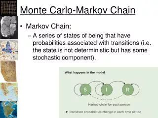
3. Markov Chain • Markov Chain • Consider chains whose transitions occur at discrete times • States S1, S2, … • Xt is the state that the chain is in at time t • Conditional probability • P(Xt=Sj|Xt1=Si1, Xt2=Si2, …, Xtn=Sin) • The system is a Markov Chain if the distribution of Xt is independent of all previous states except for its immediate predecessor Xt-1 • P(Xt=Sj|X1=Si1, X2=Si2, …, Xt-1=Sit-1)=P(Xt=Sj|Xt-1=Sit-1)

4. Characteristics of Markov Chain • Irreducible Chain • Aperiodic Chain • Stationary Distribution • Markov Chain can gradually forget its initial state • eventually converge to a unique stationary distribution • invariant distribution • Ergodic average

5. Target Distribution • Target Distribution Function • (x)=ce-h(x) • h(x) • in physics, the potential function • other system, the score function • c • normalization constant • make sure the integral of (x) is 1 • Presumably, all pdfs can be written in this form

6. Metropolis Method • Basic Idea • Evolving a Markov process to achieve the sampling of  • Metropolis Algorithm • Start with any configuration x0, iterates the following two steps • Step 1: Propose a random “perturbation” of the current state, i.e., xt -> x’, where x’ can be seen as generated from a symmetric probability transition function Q(xt->x’) • i.e., Q(x->x’)=Q(x’->x) • Calculate the change h=h(x’)-h(x) • Step 2: Generate a random number u ~ U[0, 1). Let xt+1=x’ if u<=e-h, otherwise xt+1=xt

7. Simple Example for Hard-Shell Balls • Simulation • Uniformly distributed positions of K hard-shell balls in a box • These balls are assumed to have equal diameter d • (X, Y) ={(xi, yi), i=1, …, K} • denote the positions of the balls • Target Distribution (X, Y) • = constant if the balls are all in the box and have no overlaps • =0 otherwise • Metropolis algorithm • (a) pick a ball at random, say, its position is (xi, yi) • (b) move it to a tentative position (xi’, yi’)=(xi+1, yi+2), where 1, 2 are normally distributed • (c) accept the proposal if it doesn’t violate the constraints, otherwise stay out

8. Simulation of K-Hardballs

9. Hastings’ Generalization • Metropolis Method • A symmetric transition rule • Q(x->x’)=Q(x’->x) • Hastings’ Generalization • An arbitrary transition rule • Q(x->x’) • Q() is called a proposal function

10. Metropolis-Hastings Method • Metropolis-Hastings Method • Given current state xt • Draw U ~ U[0, 1) and update • (x, y) = min{1, (y)Q(y->x)/((x)Q(x->y))}

11. Detailed Balance Condition • Transition Kernel for the Metropolis-Hastings Algorithm • I(.) denotes the indicator function • Taking the value 1 when its argument is true, and 0 otherwise • First term arises from acceptance of a candidate y=xt+1 • Second term arises from rejection, for all possible candidates y • Detailed Balance Equation • (xt)P(xt+1|xt) = (xt+1)P(xt|xt+1)

12. Gibbs Sampling • Gibbs Sampler • A special MCMC scheme • The underlying Markov Chain is constructed by using a sequence of conditional distributions which are so chosen that  is invariant with respect to each of these “conditional” moves • Gibbs Sampling • Definition • X-i={X1, …, Xi-1, Xi+1, … Xn} • Proposal Distribution • Updating the ith component of X • Qi(Xi->Yi, X-i)= (Yi|X-i)

13. MCMC Simulations • Two Phases • Equilibration • Try to reach equilibrium distribution • Measurements of steps before equilibrium are discarded • Production • After reaching equilibrium • Measurements become meaningful • Question • How fast the simulation can reach equilibrium?

14. Autocorrelations • Given a time series of N measurements from a Markov process • Estimator of the expectation value is • Autocorrelation function • Definition • where

15. Behavior of Autocorrelation Function • Autocorrelation function • Asymptotic behavior for large t • is called (exponential) autocorrelation time • is related to the second largest eigenvalue of the transition matrix • Special case of the autocorrelations

16. Integrated Autocorrelation Time Variance of the estimator Integrated autocorrelation time When

17. Reaching Equilibrium • How many steps to reach equilibrium?

18. Example of Autocorrelation Target Distribution

19. Small Step Size (d = 1)

20. Medium Step Size (d = 4)

21. Large Step Size (d = 8)

22. Microstate and Macrostate • Macrostate • Characterized by the following fixed values • N: number of particles • V: volume • E: total energy • Microstate • Configuration that the specific macrostate (E, V, N) can be realized • accessible • a microstate is accessible if its properties are consistent with the specified macrostate

23. Ensemble • System of N particles characterized by macro variables: N, V, E • macro state refers to a set of these variables • There are many micro states which give the same values of {N,V,E} or macro state. • micro states refers to points in phase space • All these micro states constitute an ensemble

24. Microcanonical Ensemble • Isolated System • N particles in volume V • Total energy is conserved • External influences can be ignored • Microcanonical Ensemble • The set of all micro states corresponding to the macro state with value N,V,E is called the Microcanonical ensemble • Generate Microcanonical Ensemble • Start with an initial micro state • Demon algorithm to produce the other micro states

25. The Demon Algorithm • Extra degree of freedom the demon goes to every particle and exchanges energy with it • Demon Algorithm • For each Monte Carlo step (for j=1 to mcs) • for i=1 to N • Choose a particle at random and make a trial change in its position • Compute E, the change in the energy of the system due to the change • If E<=0, the system gives the amount |E| to the demon, i.e., Ed=Ed- E, and the trial configuration is accepted • If E>0 and the demon has sufficient energy for this change (Ed>= E), the demon gives the necessary energy to the system, i.e., Ed=Ed- E, and the trial configuration is accepted. Otherwise, the trial configuration is rejected and the configuration is not changed

26. Monte Carlo Step • In the process of changing the micro state the program attempts to change the state of each particle. This is called a sweep or Monte Carlo Step per particle mcs • In each mcs the demon tries to change the energy of each particle once. • mcs provides a useful unit of ‘time’

27. MD and MC • Molecular Dynamic • a system of many particles with E, V, and N fixed by integrating Newton’s equations of motion for each particle • time-averaged value of the physical quantities of interest • Monte Carlo • Sampling the ensemble • ergodic-averaged value of the physical quantities of interest • How can we know that the Monte Carlo simulation of the microcanonical ensemble yields results equivalent to the time-averaged results of molecular dynamics? • Ergodic hypothesis • have not been shown identical in general • have been found to yield equivalent results in all cases of interest

28. One-Dimensional Classical Ideal Gas • Ideal Gas • The energy of a configuration is independent of the positions of the particles • The total energy is the sum of the kinetic energies of the individual particles • Interesting physical quantity • velocity • A Java Program of the 1-D Classical Ideal Gas • http://electron.physics.buffalo.edu/gonsalves/phy411-506_spring01/Chapter16/feb23.html • Using the demon algorithm

29. Physical Interpretation of Demon • Demon may be thought of as a thermometer • Simple MC simulation of ideal gas shows • Mean demon energy is twice mean kinetic of gas • The ideal gas and demon may be thought of • as a heat bath (the gas) characterized by temp T • related to its average kinetic energy • and a sub or laboratory system (the demon) • the temperature of the demon is that of the bath • The demon is in macro state T • the canonical ensemble of microstates are the Ed

30. Canonical ensemble • Normally system is not isolated. • surrounded by a much bigger system • exchanges energy with it. • Compositesystem of laboratory system and surroundings may be consider isolated. • Analogy: • lab system <=> demon • surroundings <=> ideal gas • Surroundings has temperature T which also characterizes macro state of lab system

31. Boltzmann distribution • In canonical ensemble the daemon’s energy fluctuates about a mean energy < Ed > • Probability that demon has energy Ed is given by • Boltzmann distribution • Proved in statistical mechanics • Shown by output of demon energy • Mean demon energy

32. Phase transitions • Examples: • Gas - liquid, liquid - solid • magnets, pyroelectrics • superconductors, superfluids • Below certain temperature Tc the state of the system changes structure • Characterized by order parameter • zero above Tc and non zero below Tc • e.g. magnetisation M in magnets, gap in superconductors

33. Ising model

34. Why Ising model? • Simplest model which exhibit a phase transition in two or more dimensions • Can be mapped to models of lattice gas and binary alloy. • Exactly solvable in one and two dimensions • No kinetic energy to complicate things • Theoretically and computationally tractable • can make dedicated ‘Ising machine’

35. 2-D Ising Model • E=-J • E=+J

36. Physical Quantity • Energy • Average Energy <E> • Mean Square Energy Fluctuation <(E)2>=<E2>-<E>2 • Magnetization M • Given by • mean square magnetization <(M)2>=<M2>-<M>2 • Temperature (Microcanonical)

37. Simulation of Ising Model • Microcanonical Ensemble of Ising Model • Demon Algorithm • Canonical Ensemble of Ising Model • Metropolis Algorithm

38. Metropolis for Ising Model

39. Simulating Infinite System • Simulating Infinite System • Periodic Boundaries

40. Energy Landscape • Energy Landscape • Complex biological or physical system has a complicated and rough energy landscape

41. Local Minima and Global Minima • Local Minima • The physical system may transiently reside in the local minima • Global Minima • The most stable physical/biological system • Usually the native configuration • Goal of Global Optimization • Escape the traps of local minima • Converge to the global minimum

42. Local Optimization • Local Optimization • Quickly reach a local minima • Approaches • Gradient-based Method • Quasi-Newton Method • Powell Method • Hill-climbing Method • Simplex • Global Optimization • Find the global minima • More difficult than local optimization

43. Consequences of the Occasional Ascents desired effect Help escaping the local optima. adverse effect (easy to avoid by keeping track of best-ever state) Might pass global optima after reaching it

44. Temperature is the Key • Probability of energy changes as temperature raises

45. Boltzmann distribution • At thermal equilibrium at temperature T, the Boltzmann distribution gives the relative probability that the system will occupy state A vs. state B as: • where E(A) and E(B) are the energies associated with states A and B.

46. Real annealing: Sword • He heats the metal, then slowly cools it as he hammers the blade into shape. • If he cools the blade too quickly the metal will form patches of different composition; • If the metal is cooled slowly while it is shaped, the constituent metals will form a uniform alloy.

47. Simulated Annealing Algorithm • Idea: Escape local extrema by allowing “bad moves,”but gradually decrease their size and frequency. • proposed by Kirkpatrick et al. 1983 • Simulated Annealing Algorithm • A modification of the Metropolis Algorithm • Start with any configuration x0, iterates the following two steps • Initialize T to a high temperature • Step 1: Propose a random “perturbation” of the current state, i.e., xt -> x’, where x’ can be seen as generated from a symmetric probability transition function Q(xt->x’) • i.e., Q(x->x’)=Q(x’->x) • Calculate the change h=h(x’)-h(x) • Step 2: Generate a random number u ~ U[0, 1). Let xt+1=x’ if u<=e-h/T, otherwise xt+1=xt • Step 3: Slightly reduce T and go to Step 1 Until T is your target temperature

48. Note on simulated annealing: limit cases • Boltzmann distribution: accept “bad move” with E<0 (goal is to maximize E) with probability P(E) = exp(E/T) • If T is large: E < 0 E/T < 0 and very small exp(E/T) close to 1 accept bad move with high probability • If T is near 0: E < 0 E/T < 0 and very large exp(E/T) close to 0 accept bad move with low probability Random walk Deterministic down-hill

49. Simulated Tempering • Basic Idea • Allow the temperature to go up and down randomly • Proposed by Geyers 1993 • Can be applied to a very rough energy landscape • Simulated Tempering Algorithm • At the current sampler i, update x using a Metropolis-Hastings update for i(x). • Set j = i  1 according to probabilities pi,j, where p1,2 = pm,m-1 = 1.0 and pi,i+1 = pi,i-1 = 0.5 if 1 < i < m. • Calculate the equivalent of the Metropolis-Hastings ratio for the ST method, • where c(i) are tunable constants and accept the transition from i to j with probability min(rst, 1). The distribution  is called the pseudo-prior because the function ci(x)i(x) resembles formally the product of likelihood and prior.

50. Parallel Tempering • Basic Idea • Allow multiple walks at different temperature levels • Switch configuration between temperature levels • Based on Metropolis-Hastings Ratio • Also called replica exchange method • Very powerful in complicated energy landscape