Download
1 / 39
390 likes | 576 Views
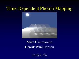
Time-Dependent Photon Mapping. Mike Cammarano Henrik Wann Jensen EGWR ‘02. Standard Photon Map. Two-pass algorithm: Photon trace Rendering. First Pass - Photon Trace. For 100 photons emitted from 100W source, each photon initially carries 1W.

E N D
Time-Dependent Photon Mapping Mike Cammarano Henrik Wann Jensen EGWR ‘02
Standard Photon Map Two-pass algorithm: • Photon trace • Rendering
First Pass - Photon Trace For 100 photons emitted from 100W source, each photon initially carries 1W. Propagate this radiant flux through scene using MC methods.
Estimating incident flux • At any patch of surface, we can estimate the incident flux: Just average the contributions of all the photons that hit the patch.
A Photon • For each surface interaction, we store: struct photon { float x,y,z; // position char power[4]; // power (RGBE) char phi, theta; // incident direction short flag; }
Photon Storage Store this information about surface interactions in photon map (kd-tree) Photon storage is decoupled from geometry
Second Pass - Rendering • Estimate flux incident at a surface point based on nearby photons.
Radiance Estimate Expand ball until it contains some reasonable number of photons. Use intersection with plane to estimate area of surface patch.
One Approach • Render lots of intermediate frames independent of one another.
Expensive • Only some areas need to be densely sampled in time. • Need MANY intermediate frames to get smooth results.
Adaptive Sampling • Want to sample densely in time only for the pixels that need it. • Easy with ray tracing. Can trace each ray for a different time in the interval. [Cook84]
Photon Map • We can’t rebuild the photon map for every eye-ray with a different time! • We would like to do DRT with photons, too. • Given rays sampling various times and photons representing lighting at various times, how do we match them up?
Photons distributed in time t=0.0t=0.5t=1.0
Energy Radiant Flux Radiant Energy
Photons in time • Want average radiance ( ∫ … dt )
Case 1 For stationary surfaces with unobstructed visibility through the entire view interval, we can ignore time distribution of photons.
Plane Moving Down t=0.0 t=0.5 t=1.0
Photon Visualization t=0.0 t=0.5 t=1.0
A Trickier Case Average of independent frames Distributed photon times t=0.0 t=0.5 t=1.0
Problem • A given patch of surface is only visible through a particular pixel for a small portion of the total time interval. • It’s brightness during that visible interval should depend only on the photons reaching it during that narrow window of time – not the “average” over all times.
Uncounted! Distribution in Time
Narrow Window in Time • Integrate over small visible interval.
Performance • Path tracing 9+ hrs • Average of independent frames 47 sec • TDPM 43 sec • Our worst case: we get essentially no benefit from adaptive sampling – doesn’t cost much to oversample blue background. • Try it in front of ~107 polygon forest …
Summary of Method IF ray-path from eye is unaffected by motion: Can integrate over entire time interval – Δt = 1. (Use all the spatially nearby photons in the estimate) ELSE Integrate over shorter visible interval. Can use several criteria for choosing Δt adaptively: 1. Δt < user-specified MaxΔt 2. Δt chosen to use only k-nearest-photons-in-time 3. Δt < time spanned by the photons
Comparison Average of 9 frames - 316 seconds
Comparison Our method – 72 seconds
Comparison Ignoring case for eye-paths with movement
Conclusion • Can incorporate correct global illumination via photon mapping in a ray-tracer that adaptively samples in time. • Computing photon map with time-dependence requires little or no added cost beyond photon mapping for the corresponding still scene. • Better performance than alternative methods for animated global illumination.