Download
1 / 14
160 likes | 437 Views
Photon Mapping. CS 319 Advanced Topics in Computer Graphics John C. Hart Featuring images swiped from Henrik Wann Jensen. Refraction of a Caustic. Monte-Carlo ray tracing handles all paths of light: L(D|S)*E, but not equally well

E N D
Photon Mapping CS 319 Advanced Topics in Computer Graphics John C. Hart Featuring images swiped from Henrik Wann Jensen
Refraction of a Caustic • Monte-Carlo ray tracing handles all paths of light: L(D|S)*E, but not equally well • Has difficulty sampling LS*DS*E paths, e.g. refraction of a caustic • Path tracing would need a very lucky first hit • Bidirectional ray tracing can find caustic, but reflection of caustic still needs lucky first hit during path tracing • Metropolis light transport can find a caustic path, but would need lucky perturbation to find its reflection
Photon Mapping • Jensen EGRW 95, 96 • Simulates the transport of individual photons • Photons emitted from light sources • Photons bounce off of specular surfaces • Photons deposited on diffuse surfaces • Held in a 3-D spatial data structure • Surfaces need not be parameterized • Photons collected by path tracing from eye
Why Map Photons? • High variance in Monte-Carlo renderings results in noise • Collection of deposited photons into a “photon map” (a 3-D spatial data structure) provides a flux density estimate • Flux samples filtered easier than path samples, resulting in error at lower frequencies • Error is a result of bias, which decreases as the number of samples increase • And, oh yeah, it’s a lot faster The scene above contains glossy surfaces, and was rendered in 50 minutes using photon mapping. The same scene took 6 hours for render with Radiance, a rendering system that used radiosity for diffuse reflection and path tracing for glossy reflection.
What is a Photon? wp • A photon p is a particle of light that carries flux DFp(xp, wp) • Power: DFp – magnitude (in Watts) and color of the flux it carries, stored as an RGB triple • Position: xp – location of the photon • Direction: wp – the incident direction wi used to compute irradiance • Photons vs. rays • Photons propogate flux • Rays gather radiance DFp xp
Sources • Point source • Photons emitted uniformly in all directions • Power of source (W) distributed evenly among photons • Flux of each photon equal to source power divided by total # of photons • For example, a 60W light bulb would send out a total of 100K photons, each carrying a flux DF of 0.6 mW • Photons sent out once per simulation, not continuously as in radiosity
Russian Roulette ? • Arvo & Kirk, S90 • Reflected flux only a fraction of incident flux • After several reflections, spending a lot of time keeping track of very little flux • Instead, completely absorb some photons and completely reflect others at full power • Spend time tracing fewer full power photons • Probability of reflectance is the reflectance r. • Probability of absorption is 1 – r. r = 60%
Mixed Surfaces • Surfaces have specular and diffuse components • rd – diffuse reflectance • rs – specular reflectance • rd + rs < 1 (conservation of energy) • Let z be a uniform random value from 0 to 1 • If z < rd then reflect diffuse • Else if z < rd + rs then reflect specular • Otherwise absorb rd = 50% rs = 30%
Storing Photons • Uses a kd-tree – a sequence of axis-aligned partitions • 2-D partitions are lines • 3-D partitions are planes • Axis of partitions alternates wrt depth of the tree • Average access time is O(log n) • Worst case O(n) when tree is severely lopsided • Need to maintain a balanced tree, which can be done in O(n log n) • Can find k nearest neighbors inO(k + log n) time using a heap
Reflected Radiance • Recall the reflected radiance equation • Convert incident radiance into incident flux • Reflected radiance in terms of incident flux • Numerically DA = pr2
DA = pr2 How Many Photons? • How big is the disk radius r? • Large enough that the disk surrounds the n nearest photons. • The number of photons used for a radiance estimate n is usually between 50 and 500. Radiance estimate using 50 photons Radiance estimate using 500 photons
Filtering • Too few photons cause blurry results • Simple averaging produces a box filtering of photons • Photons nearer to the sample should be weighted more heavily • Results in a cone filtering of photons
Multiple Photon Maps • Global L(S|D)*D photon map • Photon sticks to diffuse surface and bounces to next surface (if it survives Russian roulette) • Photons don’t stick to specular surfaces • Caustic LSS*D photon map • High resolution • Light source usually emits photons only in directions that hit the thing creating the caustic Caustic mapphotons Global mapphotons
Rendering • Rendered by glossy-surface distributed ray tracing • When ray hits first diffuse surface… • Compute reflected radiance of caustic map photons • Ignore global map photons • Importance sample BRDF fr as usual • Use global photon map to importance sample incident radiance function Li • Evaluate reflectance integral by casting rays and accumulating radiances from global photon map First diffuse intersection. Return radiance of caustic map photons here, but ignore global map photons Use global map photons to return radiance when evaluating Li at first diffuse intersection.