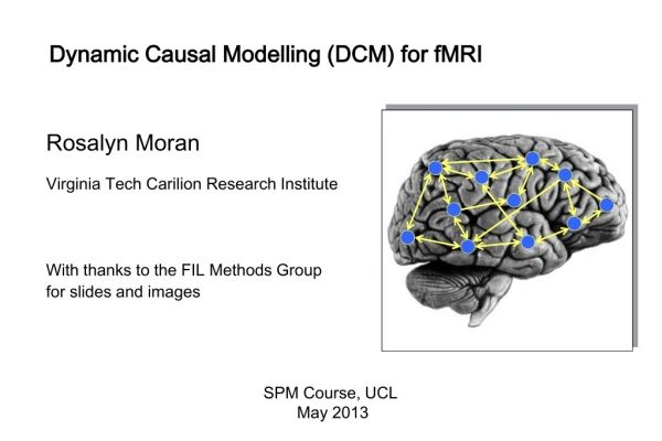
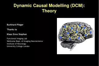
Functional Integration & Dynamic Causal Modelling (DCM)

Functional Integration& Dynamic Causal Modelling (DCM) Klaas Enno Stephan & Lee HarrisonFunctional Imaging Lab Wellcome Dept. of Imaging Neuroscience University College London ICN SPM CourseMay 6th, 2005

Overview • Classical approaches to functional & effective connectivity • Generic concepts of system analysis • DCM for fMRI: • Neural dynamics and hemodynamics • Bayesian parameter estimation • Interpretation of parameters • Statistical inference • Bayesian model selection • Practical issues and a simple example • DCM for ERPs

System analyses in functional neuroimaging Functional specialisation Analyses of regionally specific effects: which areas constitute a neuronal system? Functional integration Analyses of inter-regional effects: what are the interactions between the elements of a given neuronal system? Functional connectivity = the temporal correlation between spatially remote neurophysiological events Effective connectivity = the influence that the elements of a neuronal system exert over another MECHANISM-FREE MECHANISTIC MODEL

Functional connectivity: methods • Seed-voxel correlation analyses • Eigenimage analysis • Principal Components Analysis (PCA) • Singular Value Decomposition (SVD) • Partial Least Squares (PLS) • Independent Component Analysis (ICA)

e e Eigen-decomposition: some general maths Definition of eigenvector e and eigenvalue : Ae = e Geometric meaning: Eigenvectors are only scaled by Y; their direction is unchanged  principal axes of the matrix operation PCA: Y* = EY Re-expresses Y in terms of a new orthonormal basis E, the eigenvectors of the covariance matrix YYT. The new axes account for extreme and orthogonal components of the covariance structure. SVD: Y = USVT A general method for eigen-decomposition of matrices. If dealing with spatio-temporal data, SVD re-expresses Y in terms of the eigenvectors of the spatial and temporal covariance matrices.

SVD applied to spatio-temporal data v2T vrT v1T u2 APPROX. OF Y ur APPROX. OF Y APPROX. OF Y u1 Y (DATA) m x n matrix s1 + s2 + sr = + ... m scans n voxels ui, vi = i-th column of U and V r = rank of Y Y = USVT = s1u1v1T + s2u2v2T + ... + srurvrT U = eigenvector decomposition of YYT (temporal covariance), m x m matrix. V = eigenvector decomposition of YTY (spatial covariance), n x n matrix. S = diagonal matrix of singular values (square root of eigenvalues), m x n matrix Note: YTY and YYThave thesame non-zero eigenvalues!

SVD: an example using simulated data 128 scans A time-series of 1D images:128 scans of 40 “voxels” (note: for display reasons, the transpose of the data matrix is shown) Eigenvariates U:Temporal expression of the first three eigenimages over time Singular values S and eigenimages V ("spatial modes") The time-series reconstructed from the first three eigenimages YT 40 voxels u1…u3 v1…v3 diag(S) Y* = s1u1v1T + s2u2v2T + s3u3v3T

Pros & Cons of functional connectivity • Pros: • useful when we have no model of what caused the data (e.g. sleep, hallucinatons, etc.) • Cons: • no mechanistic insight into the neural system of interest • inappropriate for situations where we have a priori knowledge and experimental control about the system of interest models of effective connectivity necessary

Models of effective connectivity • Structural Equation Modelling (SEM) • Psycho-physiological interactions (PPI) • Multivariate autoregressive models (MAR)& Granger causality techniques • Kalman filtering • Volterra series • Dynamic Causal Modelling (DCM) now later

Psycho-physiological interaction (PPI) Task factor GLM of a 2x2 factorial design: Task B Task A main effect of task TA/S1 TB/S1 Stim 1 main effect of stim. type Stimulus factor interaction Stim 2 TB/S2 TA/S2 main effect of task We can replace one main effect in the GLM by the time series of an area that shows this main effect. E.g. let's replace the main effect of stimulus type by the time series of V1: V1 time series  main effect of stim. type psycho- physiological interaction

SPM{Z} V5 activity time V1 V5 V5 attention V5 activity no attention V1 activity PPI example: attentional modulation of V1→V5 Attention = V1 x Att. Friston et al. 1997, NeuroImage 6:218-229 Büchel & Friston 1997, Cereb. Cortex 7:768-778

V1 V5 V5 V1 attention attention PPI: interpretation Two possible interpretations of the PPI term: V1 V1 Modulation of V1V5 by attention Modulation of the impact of attention on V5 by V1.

Pros & Cons of PPIs • Pros: • given a single source region, we can test for its context-dependent connectivity across the entire brain • Cons: • very simplistic model: only allows to model contributions from a single area • ignores time-series properties of data • not easily used with event-related data • operates at the level of BOLD time series limited causal interpretability in neural terms, more powerful models needed DCM!

Models of effective connectivity = system models.But what precisely is a system? • System = set of elements which interact in a spatially and temporally specific fashion. • System dynamics = change of state vector in time • Causal effects in the system: • interactions between elements • external inputs u • System parameters  :specify the nature of the interactions • general state equation for non-autonomous systems overall system staterepresented by state variables change ofstate vectorin time

LG left FG right LG right FG left Example: linear dynamic system LG = lingual gyrus FG = fusiform gyrus Visual input in the - left (LVF) - right (RVF)visual field. z4 z3 z1 z2 RVF LVF u2 u1 systemstate input parameters state changes effective connectivity externalinputs

LG left FG right LG right FG left Extension: bilinear dynamic system z4 z3 z1 z2 CONTEXT RVF LVF u2 u3 u1

Bilinear state equation in DCM modulation of connectivity systemstate direct inputs state changes intrinsic connectivity m externalinputs

z λ y DCM for fMRI: the basic idea • Using a bilinear state equation, a cognitive system is modelled at its underlying neuronal level (which is not directly accessible for fMRI). • The modelled neuronal dynamics (z) is transformed into area-specific BOLD signals (y) by a hemodynamic forward model (λ). The aim of DCM is to estimate parameters at the neuronal level such that the modelled BOLD signals are maximally similar to the experimentally measured BOLD signals.

z λ y Conceptual overview Neural state equation The bilinear model effective connectivity modulation of connectivity Input u(t) direct inputs c1 b23 integration neuronal states a12 activity z2(t) activity z3(t) activity z1(t) hemodynamic model y y y BOLD Friston et al. 2003,NeuroImage

u 1 u 2 Z 1 Z 2 Example: generated neural data u1 u2 stimuli u1 context u2 - z1 + - Z1 z2 + + Z2 - -

The hemodynamic “Balloon” model • 5 hemodynamic parameters: important for model fitting, but of no interest for statistical inference • Empirically determineda priori distributions. • Computed separately for each area (like the neural parameters).

LG left LG right FG right FG left Example: modelled BOLD signal Underlying model(modulatory inputs not shown) left LG right LG RVF LVF LG = lingual gyrus Visual input in the FG = fusiform gyrus - left (LVF) - right (RVF) visual field. blue: observed BOLD signal red: modelled BOLD signal (DCM)

ηθ|y stimulus function u Overview:parameter estimation neural state equation • Combining the neural and hemodynamic states gives the complete forward model. • An observation model includes measurement errore and confounds X (e.g. drift). • Bayesian parameter estimationby means of a Levenberg-Marquardt gradient ascent, embedded into an EM algorithm. • Result:Gaussian a posteriori parameter distributions, characterised by mean ηθ|y and covariance Cθ|y. parameters hidden states state equation observation model modelled BOLD response

needed for Bayesian estimation, embody constraints on parameter estimation express our prior knowledge or “belief” about parameters of the model hemodynamic parameters:empirical priors temporal scaling:principled prior coupling parameters:shrinkage priors Priors in DCM Bayes Theorem posterior  likelihood ∙ prior

system stability:in the absence of input, the neuronal states must return to a stable mode → constraints on prior variance of intrinsic connections (A)→ probability <0.001 of obtaining a non-negative Lyapunov exponent (largest real eigenvalue of the intrinsic coupling matrix) shrinkage priorsfor coupling parameters (η=0)→ conservative estimates! Priors in DCM • self-inhibition:ensured by priors on the decay rate constant σ (ησ=1, Cσ=0.105)→ these allow for neural transients with a half life in the range of 300 ms to 2 secondsNB: a single rate constant for all regions! • Identical temporal scaling in all areas by factorising A and B with σ: all connection strengths are relative to the self-connections.

Shrinkage Priors Small & variable effect Large & variable effect Small but clear effect Large & clear effect

ηθ|y Parameter estimation in DCM • Bayesian parameter estimation under Gaussian assumptions by means of EM and gradient ascent. • Result:Gaussian a posteriori parameter distributions, characterised by mean ηθ|y and covariance Cθ|y. • Combining the neural and hemodynamic states gives the complete forward model: • The observation model includes measurement error and confounds X (e.g. drift):

Bayesian estimation: univariate Gaussian case Normal densities Univariate linear model Relative precision weighting

Bayesian estimation: multivariate Gaussian case General Linear Model Normal densities One step if Ce is known.

Current estimates Local linearization by 1st order Taylor: Likelihood Gradient ascent (Fisher scoring) with priors Friston (2002) NeuroImage, 16: 513-530. Bayesian estimation: nonlinear case Prior density

EM and gradient ascent • Bayesian parameter estimation by means of expectation maximisation (EM) • E-step:gradient ascent (Fisher scoring & Levenberg-Marquardt regularisation) on the log posterior to compute • (i) the conditional mean ηθ|y(= expansion point of gradient ascent), • (ii) the conditional covariance Cθ|y • M-step:ReML estimates of hyperparameters ifor error covariance components Qi: • Note: Gaussian assumptions about the posterior (Laplace approximation)

E-step: Fisher scoring Generally, Fisher scoring is identical to the Gauss-Newton algorithm (except that the expectation of the Hessian is taken): For DCM, the Fisher scoring scheme can be derived by taking partial derivatives of the log posterior wrt. to the parameters: This results in equations equivalent to those derived for posterior mode estimation in non-linear cases, using local linearisation (see previous slides) :

E-step: Levenberg-Marquardt regularisation For updating the parameters in the E-step, an LM regularisation ensures a good balance between steepest gradient ascent and Gauss-Newton ascent. steepest gradient ascentlarge step for large gradient  risk of overshooting a maximum small steps for small gradients  slow progress in “uninteresting” areas Gauss-Newton algorithmderived from 2nd order Taylor expansion  quadratic assumption about local properties of objective function Levenberg algorithmdynamically adjusts :small   Gauss-Newtonlarge   steepest gradient ascent Levenberg-Marquardt algorithm:makes use of curvature even if  is high:scales each component of the gradient according to the curvature

Parameter estimation (new):output in command window E-Step: 1 F: -1.514001e+003 dp: 8.299907e-002 E-Step: 2 F: -1.200724e+003 dp: 9.638851e-001 E-Step: 3 F: -1.115951e+003 dp: 2.703493e-001 E-Step: 4 F: -1.077757e+003 dp: 2.002973e-002 E-Step: 5 F: -1.075699e+003 dp: 4.219233e-003 E-Step: 6 F: -1.075663e+003 dp: 1.030322e-003 E-Step: 7 F: -1.075661e+003 dp: 3.595806e-004 E-Step: 8 F: -1.075661e+003 dp: 2.273264e-006 Change of the norm of the parameter vector (= magnitude of update) objective function

DCM parameters = rate constants Generic solution to the ODEs in DCM: Decay function: Half-life:

Inference about DCM parameters:Bayesian single-subject analysis • Bayesian parameter estimation in DCM: Gaussian assumptions about the posterior distributions of the parameters • Use of the cumulative normal distribution to test the probability by which a certain parameter (or contrast of parameters cT ηθ|y) is above a chosen threshold γ: • γ can be chosen as zero ("does the effect exist?") or as a function of the expected half life τ of the neural process: γ= ln 2 / τ  ηθ|y

Inference about DCM parameters: Bayesian fixed-effects group analysis Because the likelihood distributions from different subjects are independent, one can combine their posterior densities by using the posterior of one subject as the prior for the next: Under Gaussian assumptions this is easy to compute: group posterior covariance individual posterior covariances group posterior mean individual posterior covariances and means See: spm_dcm_average.m Neumann & Lohmann, NeuroImage 2003

Inference about DCM parameters:group analysis (classical) • In analogy to “random effects” analyses in SPM, 2nd level analyses can be applied to DCM parameters: Separate fitting of identical models for each subject Selection of bilinear parameters of interest one-sample t-test:parameter > 0 ? paired t-test:parameter 1 > parameter 2 ? rmANOVA:e.g. in case of multiple sessions per subject

Pitt & Miyung (2002), TICS Model comparison and selection Given competing hypotheses on structure & functional mechanisms of a system, which model is the best? For which model i does p(y|mi) become maximal? Which model represents the best balance between model fit and model complexity?

Bayes theorem: Model evidence: The log model evidence can be represented as: Bayes factor: Bayesian Model Selection Penny et al. 2004, NeuroImage

Laplace approximation: Akaike information criterion (AIC): Bayesian information criterion (BIC): Approximations to model evidence Unfortunately, the complexity term depends on the prior density, which is determined individually for each model to ensure stability. Therefore, we need other approximations to the model evidence. Penny et al. 2004, NeuroImage

Hypothesis abouta neural system The DCM cycle Statistical test on parameters of optimal model Definition of DCMs as systemmodels Bayesian modelselection of optimal DCM Design a study thatallows to investigatethat system Parameter estimationfor all DCMs considered Data acquisition Extraction of time seriesfrom SPMs

Planning a DCM-compatible study • Suitable experimental design: • preferably multi-factorial (e.g. 2 x 2) • e.g. one factor that varies the driving (sensory) input • and one factor that varies the contextual input • TR: • as short as possible (optimal: < 2 s) • Hypothesis and model: • define specific a priori hypothesis • which parameters are relevant to test this hypothesis? • ensure that intended model is suitable to test this hypothesis → simulations before experiment • define criteria for inference

Timing problems at long TRs • Two potential timing problems in DCM: • wrong timing of inputs • temporal shift between regional time series because of multi-slice acquisition 2 slice acquisition 1 visualinput • DCM is robust against timing errors up to approx. ± 1 s • compensatory changes of σ and θh • Possible corrections: • slice-timing (not for long TRs) • restriction of the model to neighbouring regions • in both cases: adjust temporal reference bin in SPM defaults (defaults.stats.fmri.t0)

Practical steps of a DCM study - I • Conventional SPM analysis (subject-specific) • DCMs are fitted separately for each session → consider concatenation of sessions or adequate 2nd level analysis • Definition of the model (on paper!) • Structure: which areas, connections and inputs? • Which parameters represent my hypothesis? • How can I demonstrate the specificity of my results? • What are the alternative models to test? • Defining criteria for inference: • single-subject analysis: stat. threshold? contrast? • group analysis: which 2nd-level model?

Practical steps of a DCM study - II • Extraction of time series, e.g. via VOI tool in SPM • cave: anatomical & functional standardisation important for group analyses! • Possibly definition of a new design matrix, if the “normal” design matrix does not represent the inputs appropriately. • NB: DCM only reads timing information of each input from the design matrix, no parameter estimation necessary. • Definition of model • via DCM-GUI or directlyin MATLAB

Practical steps of a DCM study - III • DCM parameter estimation • cave: models with many regions & scans can crash MATLAB! • Model comparison and selection: • Which of all models considered is the optimal one? Bayesian model selection tool • Testing the hypothesisStatistical test onthe relevant parametersof the optimal model

Attention to motion in the visual system Stimuli 250 radially moving dots at 4.7 degrees/s Pre-Scanning 5 x 30s trials with 5 speed changes (reducing to 1%) Task - detect change in radial velocity Scanning(no speed changes) 6 normal subjects, 4 x 100 scan sessions; each session comprising 10 scans of 4 different conditions F A F N F A F N S ................. F - fixation point only A - motion stimuli with attention (detect changes) N - motion stimuli without attention S - no motion PPC V3A V5+ Attention – No attention Büchel & Friston 1997, Cereb. Cortex Büchel et al.1998, Brain

Functional Integration & Dynamic Causal Modelling (DCM)