Download
1 / 15
160 likes | 376 Views
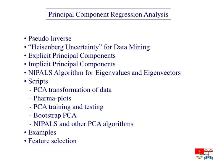
Principal Component Regression Analysis. • Pseudo Inverse • “Heisenberg Uncertainty” for Data Mining • Explicit Principal Components • Implicit Principal Components • NIPALS Algorithm for Eigenvalues and Eigenvectors • Scripts - PCA transformation of data - Pharma-plots

E N D
Principal Component Regression Analysis • Pseudo Inverse • “Heisenberg Uncertainty” for Data Mining • Explicit Principal Components • Implicit Principal Components • NIPALS Algorithm for Eigenvalues and Eigenvectors • Scripts - PCA transformation of data - Pharma-plots - PCA training and testing - Bootstrap PCA - NIPALS and other PCA algorithms • Examples • Feature selection
( ) - 1 T T X X X mn nm mn Classical Regression Analysis Pseudo inverse Penrose inverse Least-Squares Optimization
( ) - 1 T X X The Machine Learning Paradox If data are can learned from, they must have redundancy If there is redundancy, (XTX)-1 is ill-conditioned - similar data patterns - closely correlated descriptive features
» X T B nm nh hm = T T X B nh nm mh Beyond Regression • Paul Werbos motivated beyond regression in 1972 • In addition, there are related statistical “duals” (PCA, PLS, SVM) • Principal component analysis: h = # Principal components • Trick: eliminate poor conditioning by using h PC’s (largest ) • Now matrix to invert is small and well-conditioned • Generally include ~ 2 - 4 -6 PCAs • A Better PCA Regression is PLS (Please Listen to Savanti Wold) • A Better PLS is nonlinear PNLS
» X T B nm nh hm = T T X B nh nm mh Explicit PCA Regression • We had • Assume we derive PCA features for A according to • We now have h = # Principal components
Explicit PCA Regression on training/test set • We have for training set: • And for the test set:
» X T B nm nh hm = T T X B nh nm mh Implicit PCA Regression h = # Principal components How to apply? Calculate T and B with NIPALS algorithm Determine b, and apply to data matrix
» X T B nm nh hm = T T X B nh nm mh Algorithm h = # Principal components • The B matrix is a matrix of eigenvectors of the correlation matrix C • If the features are zero centered we have: • We only consider the h eigenvectors corresponding to largest eigenvalues • The eigenvalues are the variances • Eigenvectors are normalized to 1 and solutions of: • Use NIPALS algorithm to build up B and T
» X T B nm nh hm = T T X B nh nm mh NIPALS Algorithm: Part 2 h = # Principal components
PRACTICAL TIPS FOR PCA • NIPALS algorithm assumes the features are zero centered • It is standard practice to do a Mahalanobis scaling of the data • PCA regression does not consider the response data • The t’s are called the scores • Use 3-10 PCA’s • I usually use 4 PCA’s • It is common practice to drop 4 sigma outlier features • (if there are many features)
PCA with Analyze • Several options: option #17 for training and #18 for testing • (the weight vectors after training is in file bbmatrixx.txt) • The file num_eg.txt contains a number equal to # PCAs • Option –17 is the NIPALS algorithm and generally faster than 17 • SAnalyze has options for calculating T’s, B’s and ’s • - option #36 transforms a data matrix to it’s PCAs • - option #36 also saves eigenvalues and eigenvectors of XTX • Analyze has also option for bootstrap PCA (-33)
StripMiner Scripts • last lecture: iris_pca.bat (make PCAs and visualize) • iris.bat (split up data in training and validation set and predict) • iris_boot.bat (bootstrap prediction)
Bootstrap Prediction (iris_boo.bat) • Make different models for training set • Predict Test set on average model
PCA in DATA SPACE Means that the similarity score with each data point will be weighed (i.e.., effectively incorporating Mahalanobis scaling in data space) Σ Σ x1 This layer gives a similarity score with each datapoint Σ Σ . . . Σ Σ Σ xi Σ Σ Kind of a nearest neighbor weighted prediction score xM Σ Weights correspond to H eigenvectors corresponding to largest eigenvalues of XTX Weights correspond to the dependent variable for the entire training data Σ Weights correspond to the scores or PCAs for the entire training set